
Sorting refers to arranging data in a systematic order, either in ascending or descending order. A Sorting Algorithm is used to rearrange a given array or list of elements by comparing the elements based on some operator. The comparison operator is used to decide the new order of elements in the respective data structure.

There are various types of sorting algorithms in python:
- Bubble Sort
- Selection Sort
- Insertion Sort
- Bucket Sort
- Merge Sort
- Quick Sort
- Heap Sort
- Tree Sort
- Shell Sort
- Count Sort
- Radix Sort
Example – A list of unsorted elements

List after sorting

Types of Sorting Algrorithms
Based on Space Used
In place Sorting Algorithm
In-place sorting algorithms are algorithms that do not require any extra space for sorting. This means that no other data structure is used to store data, even temporarily. However, a small amount of extra storage space is allowed for auxiliary variables. Example: Bubble Sort.
Out place Sorting Algorithm
Out-place sorting algorithms are algorithms that require extra spacing for sorting. These algorithms require a separate data structure to insert values into and then implement sorting. The size of the data structure depends on the input size. Example: Merge Sort.
Based on Stability
Stable Sorting Algorithm
If a sorting algorithm, after sorting the contents, does not change the sequence of similar content in which they appear, then this algorithm is called a stable sorting algorithm.
This means that if there are two elements in a list with values of 40 each, then after sorting, they are going to be placed adjacent to each other in the same order as they were before Example: Insertion Sort
Unstable Sorting Algorithm
If a sorting algorithm, after sorting the contents, changes the sequence of similar content in which they appear, then this algorithm is called an unstable sorting algorithm.
ts in a list with values of 80 each, then after sorting, they are going to be placed adjacent to each other in a different order as they were before Example: Quick Sort
Sorting Terminologies
- Increasing Order – If the successive element in a sorted array is greater than the previous one, then they are said to be arranged in an increasing order.
Example: 1, 3, 5, 7, 9, 11 - Decreasing Order – If the successive element in a sorted array is lesser than the previous one, then they are said to be arranged in a decreasing order.
Example: 11, 9, 7, 5, 3, 1 - Non Increasing Order – If the successive element in a sorted array is lesser than or equal to the previous one, then they are said to be arranged in a non increasing order.
Example: 11, 9, 7, 5, 5, 3, 1 - Non Decreasing Order – If the successive element in a sorted array is greater than or equal to the previous one, then they are said to be arranged in a non decreasing order.
Example: 1, 3, 5, 7, 7, 9, 11
We determine our choice of sorting algorithm based on the following three factors:
- Stability
- Time Efficiency
- Space Efficiency
Important Sorting Algorithms in Python
Bubble Sort
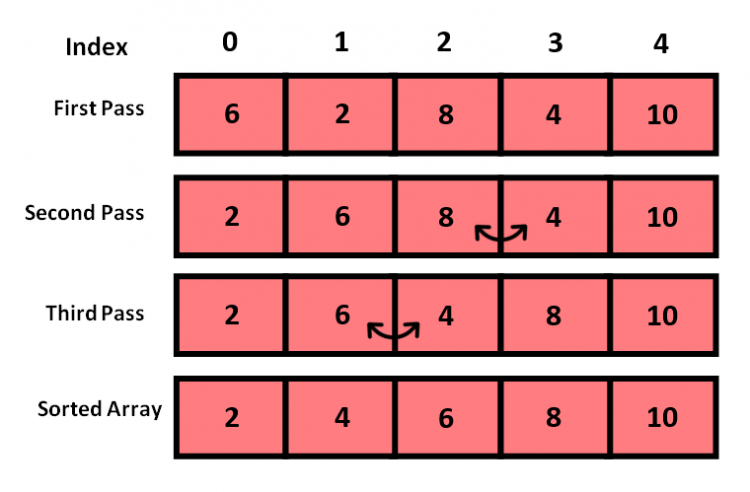
Bubble sort is a simple sorting algorithm that repeatedly steps through the list, compares adjacent elements, and swaps them if they are in the wrong order. Each iteration in a bubble sort algorithm is called a pass. The pass of the list is repeated until the list is sorted.
After every iteration in Bubble Sort Algorithm, the largest number in the unsorted list gets placed at the right position. Hence, it is also called Sinking Sort.
Implementation of Bubble Sort Algortihm
The implementation of the Bubble Sort is based on the following algorithm:
- We set a for loop to iterate over each element of the list.
- Within this for loop, we put a nested for loop to iterate through the remaining unsorted list after each pass.
- Values of adjacent elements are compared at each iteration and they are swapped if they are in the wrong order.
#Function to implement Bubble Sort
def bubbleSort(tempList):
    for i in range(len(tempList)-1):
        for j in range(len(tempList)-i-1):
            if tempList[j] > tempList[j+1]:
                tempList[j], tempList[j+1] = tempList[j+1], tempList[j]
    print(tempList)

unsortedList = [6, 2, 8, 4, 10]
bubbleSort(unsortedList)

#Output
[2, 4, 6, 8, 10]
Time and Space Complexity
The time complexity for the bubble sort algorithm is O(N2) because it works on a nested for loop which iterates through the list for each separate element. The space complexity is O(1) as no additional memory is required.
When to use or avoid Bubble Sort
When to use Bubble Sort:
- To check if a given list if fully sorted.
- When space is a concern, bubble sort provides good space complexity
- It is a simple, easy to implement algorithm and can be used for sorting small number of elements.
When to avoid Bubble Sort:
- The average time complexity for bubble sort is quite poor. Thus, we avoid using it for sorting lists of bigger sizes.
Selection Sort
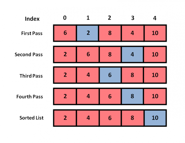
The selection sort algorithm sorts a list by repeatedly finding the minimum element from the unsorted part and putting it at the beginning. The algorithm maintains two subarrays in a given array.
- The sublist that is already sorted.
- Remaining sublist which is unsorted.
In every iteration of selection sort, the minimum element of the unsorted sublist is picked and moved to the sorted sublist.
Implementation of Selection Sort Algortihm
The implementation of the Selection Sort is based on the following algorithm:
- We set a for loop to iterate over each element of the list.
- Within this for loop, we put a nested for loop to iterate through the remaining list and find the minimum value in the unsorted list.
- The least value in the unsorted list, after each pass, is placed at its correct position.
#Function to implement Selection Sort
def selectionSort(tempList):
    for i in range(len(tempList)):
        min_index = i
        for j in range(i+1, len(tempList)):
            if tempList[min_index] > tempList[j]:
                min_index = j
        tempList[i], tempList[min_index] = tempList[min_index], tempList[i]
    print(tempList)

unsortedList = [6, 2, 8, 4, 10]
selectionSort(unsortedList)

#Output
[2, 4, 6, 8, 10]
Time and Space Complexity
The time complexity for the selection sort algorithm is O(N2) because it works on a nested for loop which iterates through the list for each separate element. The space complexity is O(1) as no additional memory is required.
When to use or avoid Selection Sort
When to use Selection Sort:
- When we have insufficient memory and need a space efficient algorithm.
- It is a simple, easy to implement algorithm and can be used for sorting small number of elements.
When to avoid Selection Sort:
- The average time complexity for selection sort is quite poor. Thus, we avoid using it for sorting lists of bigger sizes.
Insertion Sort
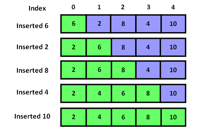
Insertion Sort is a simple sorting algorithm that sorts an array or list one item at a time. The list is virtually split into two parts – the sorted part and the unsorted part. Data values are picked from the unsorted part and placed at their correct position in the sorted part.
For example, when sorting a deck of playing cards, we insert each card into its right position one by one until the deck is fully sorted. Insertion sort works in the exact same manner.
Implementation of Insertion Sort Algortihm
The implementation of the Insertion Sort is based on the following algorithm:
- Iterate from the first element of the list to the last.
- Compare the current element, i.e., the key element to its predecessor.
- If the key element is smaller than its predecessor, compare it to the elements before that. Move the greater elements one position up to make space for the swapped element and place the key at its rightful place in the list.
#Function to implement Insertion Sort
def insertionSort(tempList):
    for i in range(1, len(tempList)):
        key = tempList[i]
        j = i-1
        while j >= 0 and key < tempList[j]:
            tempList[j+1] = tempList[j]
            j -= 1
        tempList[j+1] = key
    return tempList

unsortedList = [6, 2, 8, 4, 10]
print(insertionSort(unsortedList))

#Output
[2, 4, 6, 8, 10]
Time and Space Complexity
The time complexity for the insertion sort algorithm is O(N2) because it works on a nested loop that iterates through the list for each separate element. The space complexity is O(1) as no additional memory is required.
When to use or avoid Insertion Sort
When to use Insertion Sort:
- When we have insufficient memory and need a space efficient algorithm.
- It is a simple, easy to implement algorithm and can be used for sorting small number of elements.
- When we have continuous inflow of numbers and we want to keep them sorted.
When to avoid Insertion Sort:
- The average time complexity for insertion sort is quite poor. Thus, we avoid using it for sorting lists of bigger sizes.
Bucket Sort
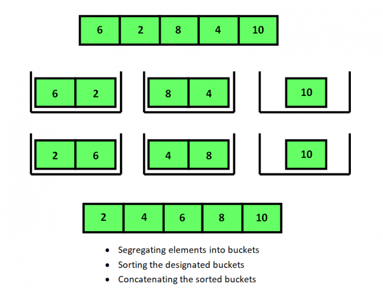
Bucket Sort is a sorting algorithm that segregates the unsorted elements of a list or array into several groups called buckets. Each bucket is then sorted by using any of the suitable sorting algorithms or recursively calling the same bucketSort algorithm.
Finally, all the sorted buckets are combined to create the final sorted list. We will use the insertionSort method to sort the unsorted buckets.
Implementation of Bucket Sort Algortihm
The implementation of the Bucket Sort is based on the following algorithm:
- Partition the given list into n non-overlapping buckets where n equals
round(math.sqrt(len(tempList))). - Insert each input number into its bucket.
- Sort each bucket using the
insertionSortalgorithm. - Concatenate the sorted buckets to form the sorted list.
#Function to implement Bucket Sort
def bucketSort(tempList):
    numberofBuckets = round(math.sqrt(len(tempList)))
    maxVal = max(tempList)
    arr = []

    for i in range(numberofBuckets):
        arr.append([])
    for j in tempList:
        index_b = math.ceil(j*numberofBuckets/maxVal)
        arr[index_b-1].append(j)

    for i in range(numberofBuckets):
        arr[i] = insertionSort(arr[i])

    k = 0
    for i in range(numberofBuckets):
        for j in range(len(arr[i])):
            tempList[k] = arr[i][j]
            k += 1
    return tempList

unsortedList = [6, 2, 8, 4, 10]
print(bucketSort(unsortedList))

#Output
[2, 4, 6, 8, 10]
Time and Space Complexity
The time complexity for the bucket sort algorithm is O(N2) because it uses insertion sort to order the elements of each individual bucket. The space complexity is O(N) as an extra data structure is required as buckets to hold the elements.
When to use or avoid Bucket Sort
When to use Bucket Sort:
- When the input is uniformly distributed over a given a range.
When to avoid Bucket Sort:
- Bucket Sort takes an extra space to create the designated buckets and thus it is not a space efficient algorithm. Its use should be avoided when space is a concern.
Merge Sort
Merge Sort is based on the Divide and Conquer Algorithm. It divides the input list into two halves, calls itself recursively for the two halves, and then merges the two sorted halves. Here, a problem is divided into multiple sub-problems. Each sub-problem is solved individually. Finally, sub-problems are combined to form the final solution.
The merge function is used for merging the two halves. The merge(arr, left, middle, right) method is a key process that assumes that list[left..middle] and list[middle+1..right] are sorted and merges the two sorted sub-lists into one.

Implementation of Merge Sort Algortihm
For the merge sort algorithm, we recursively follow these steps till the right variable passed to merge is greater than the left variable.
- We find the middle point to divide the array into two halves.
- The
mergeSortmethod is called for the first half. - Then, the
mergeSortmethod is called for the second half. - Finally, we merge the two halves using the
mergefunction.
#Function to implement Merge Sort
def merge(tempList, left, middle, right):
    n1 = middle - left + 1
    n2 = right - middle

    L = [0] * (n1)
    R = [0] * (n2)

    for i in range(0, n1):
        L[i] = tempList[left+i]

    for j in range(0, n2):
        R[j] = tempList[middle+1+j]

    i = 0
    j = 0
    k = left
    while i < n1 and j < n2:
        if L[i] <= R[j]:
            tempList[k] = L[i]
            i += 1
        else:
            tempList[k] = R[j]
            j += 1
        k += 1
    while i < n1:
        tempList[k] = L[i]
        i += 1
        k += 1

    while j < n2:
        tempList[k] = R[j]
        j += 1
        k += 1


def mergeSort(tempList, left, right):
    if left < right:
        middle = (left+(right-1))//2
        mergeSort(tempList, left, middle)
        mergeSort(tempList, middle+1, right)
        merge(tempList, left, middle, right)
    return tempList

unsortedList = [6, 2, 8, 4, 10]
print(mergeSort(unsortedList, 0, 4))

#Output
[2, 4, 6, 8, 10]
Time and Space Complexity
The merge sort algorithm recursively divides the list into halves till they are broken into single elements which take O(logN) time, and the merge function recombines them with a time of O(N). Thus, the time complexity takes the form of O(NlogN). The space complexity is O(N) as an extra data structure is required to hold the unsorted elements.
When to use or avoid Merge Sort
When to use Merge Sort:
- When there is a need of a stable sorting algorithm, merge sort can be implemented.
- The average time complexity is O(NlogN) which is comparitively lesser than other algorithms.
When to avoid Merge Sort:
- The merge function creates sub-arrays which takes up space in the memory. Hence, merge sort algorithm can be avoided when space efficiency is a concern.
Quick Sort
Similar to Merge Sort, Quick Sort is a Divide and Conquer Algorithm. It picks an element as a pivot and partitions the given list around the chosen pivot. According to the pivot selected, Quick Sort can be divided into these categories:
- First element is always selected as the pivot.
- Last element is always selected as the pivot.
- A random element is selected as the pivot.
- The median of the list is selected as the pivot.
The partition method performs an important process in the implementation of Quick Sort. The function picks the pivot of the list and places it at its correct position. Then, the elements smaller than the pivot are placed to its left, and the elements greater than the pivot are placed to its right.

Implementation of Quick Sort Algortihm
The Quick Sort Algorithm is based on the following steps:
- Set a pivot to partition the given list.
- Place elements smaller than the pivot to its left.
- Place elements greater than the pivot to its right.
- Continue this process for the sub-lists untill the last element of each iteration.
#Function to implement Quick Sort
def partition(tempList, low, high):
    i = low - 1
    pivot = tempList[high]
    for j in range(low, high):
        if tempList[j] <= pivot:
            i += 1
            tempList[i], tempList[j] = tempList[j], tempList[i]
    tempList[i+1], tempList[high] = tempList[high], tempList[i+1]
    return (i+1)


def quickSort(tempList, low, high):
    if low < high:
        pi = partition(tempList, low, high)
        quickSort(tempList, low, pi-1)
        quickSort(tempList, pi+1, high)

unsortedList = [4, 2, 10, 8, 6]
quickSort(unsortedList, 0, 4)
print(unsortedList)

#Output
[2, 4, 6, 8, 10]
Time and Space Complexity
The Quick Sort Algorithm recursively divides the list into halves till they are broken into single elements which take O(logN) time, and any sort function is used to sort the sub-lists and recombine them simultaneously with a time of O(N). Thus, the time complexity takes the form of O(NlogN). The space complexity is O(N) as an extra data structure is required to hold the unsorted elements.
When to use or avoid Quick Sort
When to use Quick Sort:
- The average time complexity is O(NlogN) which is comparitively lesser than other algorithms. Quick Sort can be used to save time.
When to avoid Quick Sort:
- The quick sort function creates sub-arrays which takes up space in the memory. Hence, quick sort algorithm can be avoided when space efficiency is a concern.
- Quick Sort Algorithm is not a stable algorithm and can be avoided.
Heap Sort
A binary heap is a binary tree that is complete, i.e., all levels of the tree are filled except possibly the last level and the leaf nodes are as far left as possible. A binary heap is either a min-heap or a max-heap.
In a Min Binary Heap, the key at the root must be minimum among all keys present in Binary Heap. The same property must be recursively true for all nodes in Binary Heap Tree. Max Binary Heap is similar to MinHeap wherein all root nodes hold the max value among their children.
Heap Sort is a comparison-based sorting algorithm that makes use of a binary heap for sorting the elements. It is similar to selection sort where the minimum element is found in the list and placed at the beginning. This process is then continued until all elements are placed at their rightful position.

Implementation of Heap Sort Algortihm
The Heap Sort Algorithm is based on the following steps:
- Insert the values of the unsorted array into the heap data structure.
- Use the
heapifyfunction to heapify the tree into a min heap tree. - Finally, insert the sorted values from the binary heap into the list.
#Function to implement Heap Sort
def heapify(tempList, n, i):
    smallest = i
    left = 2*i + 1
    right = 2*i + 2
    if left < n and tempList[left] < tempList[smallest]:
        smallest = left

    if right < n and tempList[right] < tempList[smallest]:
        smallest = right

    if smallest != i:
        tempList[i], tempList[smallest] = tempList[smallest], tempList[i]
        heapify(tempList, n, smallest)


def heapSort(tempList):
    n = len(tempList)
    for i in range(int(n/2)-1, -1, -1):
        heapify(tempList, n, i)

    for i in range(n-1, 0, -1):
        tempList[i], tempList[0] = tempList[0], tempList[i]
        heapify(tempList, i, 0)
    tempList.reverse()

unsortedList = [6, 2, 8, 4, 10]
heapSort(unsortedList)
print(unsortedList)

#Output
[2, 4, 6, 8, 10]
Time and Space Complexity
The method heapify takes O(logN) for each function call and it is called with every node insertion. Hence, the overall time complexity for Heap Sort Algorithm is O(NlogN). The space complexity Is O(1) as no additional memory is required.
When to use or avoid Heap Sort
When to use Heap Sort:
- Heap Sort is an in-place sorting algorithm and provides better space efficiency. Hence, it can be used where space is a concern.
When to avoid Heap Sort:
- Heap Sort is less efficient than Quick Sort in most of the cases and hence can be avoided.
Count Sort
Count Sort or Counting Sort is a sorting algorithm that sorts the elements of a list or array by counting and storing the number of occurrences of each distinct element of the array. Subsequently, we perform some arithmetic calculations to find the position of each object in the sorted output list.
Implementation of Count Sort Algortihm
The Count Sort Algorithm is based on the following steps:
- Find the element with the maximum value(max). Initialize an array “count” with size max+1 with all elements set to 0.

- Store the number of occurences for each element at their respective index in the “count” array.

- Store the cumulative sum of the elements of the count array. Later, this well help in positioning them in the output arrray.

- Find the index of each element of the original array in the count array. This gives the cumulative count. Subtract 1 to get the index of that element in the sorted array.

#Function to implement Count Sort
def countSort(tempList):
    size = len(tempList)
    resultList = [0] * size
    maxNo = max(tempList)
    sizeOfCount = maxNo + 1
    countList = [0] * sizeOfCount

    for i in range(0, size):
        countList[tempList[i]] += 1

    for i in range(1, sizeOfCount):
        countList[i] += countList[i - 1]

    i = size - 1
    while i >= 0:
        resultList[countList[tempList[i]] - 1] = tempList[i]
        countList[tempList[i]] -= 1
        i -= 1

    for i in range(0, size):
        tempList[i] = resultList[i]


unsortedList = [4, 2, 5, 3, 6, 3]
countSort(unsortedList)
print(unsortedList)

#Output
[2, 3, 3, 4, 5, 6]
Output:

Time and Space Complexity
The count sort algorithm uses four loops – two of time complexities O(max) and two of time complexities O(size). The final time complexity is O(max + size). The space complexity Is O(max) as we create an extra list data structure of size “max”.
When to use or avoid Count Sort
When to use Count Sort:
- Count Sort algorithm is used when time is a concern as it provides linear time complexity.
When to avoid Count Sort:
- Count Sort needs extra space in memory to implement. Hence, it can be avoided when sorting arrays of significantly bigger sizes.
Radix Sort
Radix sort is a sorting algorithm that sorts the elements by grouping individual digits of the same place value. Then, the elements are sorted according to their increasing/decreasing order.
Suppose, we have an unsorted array or list. Firstly, we will sort the elements of the list based on the value of the unit place. Then, we will sort the elements based on the value of the tenth place. The same process is carried on till we sort the last significant place.
Implementation of Radix Sort Algortihm
The Radix Sort Algorithm is based on the following steps:
- We find the largest number in the unsorted list or array. We then store the number of digits of this element so that we recognize the last significant digit.

- We go through each significant value place one by one. Then, we use the count sort algorithm to sort the digits at each significant place.


- Keep sorting the digits at each significant place untill the last significant place has been sorted. This gives us the sorted array.

#Function to implement Radix Sort
def countSort(tempList, place):
    size = len(tempList)
    resultList = [0] * size
    maxNo = max(tempList)
    sizeOfCount = maxNo + 1
    countList = [0] * sizeOfCount

    for i in range(0, size):
        index = tempList[i] // place
        countList[index % 10] += 1

    for i in range(1, sizeOfCount):
        countList[i] += countList[i - 1]

    i = size - 1
    while i >= 0:
        index = tempList[i] // place
        resultList[countList[index % 10] - 1] = tempList[i]
        countList[index % 10] -= 1
        i -= 1

    for i in range(0, size):
        tempList[i] = resultList[i]


def radixSort(tempList):
    max_element = max(tempList)

    place = 1
    while max_element // place > 0:
        countSort(tempList, place)
        place *= 10


unsortedList = [121, 432, 564, 23, 1, 45, 788]
radixSort(unsortedList)
print(unsortedList)

#Output
[1, 23, 45, 121, 432, 564, 788]
Time and Space Complexity
The time complexity for the radix sort algorithm is O(dig(size+max)) where O(size+max) is the time complexity of count sort and dig is the maximum number of significant digits place. The space complexity Is O(max) as we create an extra list data structure of size “max”.
When to use or avoid Radix Sort
When to use Radix Sort:
- Radix Sort algorithm is used when time is a concern as it provides linear time complexity, which is lesser than O(NlogN).
When to avoid Radix Sort:
- Radix Sort needs extra space in memory to implement. Hence, it can be avoided when sorting arrays of significantly bigger sizes.
Shell Sort
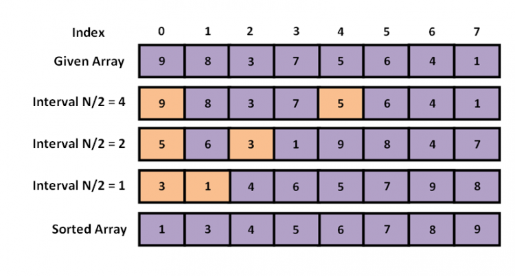
The Shell Sort Algorithm is similar to insertion sort. It sorts elements that are far away from each other and consequently decreases the gap between the elements to be sorted.
We use several sequences to reduce the interval between the elements to be sorted. We will use Shell’s original sequence(N/2, N/4, ……….., 1) for the implementation of the Shell Sort Algorithm.
Implementation of Shell Sort Algortihm
The Shell Sort Algorithm is based on the following steps:
- Suppose, we receive an unsorted list of length equal to 8.
- In the first iteration, N/2 = 4. Hence, we compare the element at the 0th index with the one at 4th, the element at the 1st index with the one at 5th, and so on.
- In the next iteration, the gap between elements is reduced to 2. Thus, we compare elements at intervals of 2 and swap them if they are placed in the wrong order.
- In the last iteration, when the interval reduces to 1, we sort the elements at adjacent places and receive the final output list.
#Function to implement Shell Sort
def shellSort(tempList, n):
    interval = n // 2
    while interval > 0:
        for i in range(interval, n):
            tempNo = tempList[i]
            j = i
            while j >= interval and tempList[j - interval] > tempNo:
                tempList[j] = tempList[j - interval]
                j -= interval

            tempList[j] = tempNo
        interval //= 2


unsortedList = [9, 8, 3, 7, 5, 6, 4, 1]
sizeOfList = len(unsortedList)
shellSort(unsortedList, sizeOfList)
print(unsortedList)

#Output
[1, 3, 4, 5, 6, 7, 8, 9]
Time and Space Complexity
The time complexity for Shell Sort is O(NlogN) as we divide the given list into fragments based on the intervals. We do this for every iteration and then compare elements. The space complexity is O(1) as no additional memory is required.
When to use or avoid Shell Sort
When to use Shell Sort:
- Shell Sort is used in cases where space is a concern. It does not require any extra data structure for temporarily storing the elements.
When to avoid Shell Sort:
- Shell Sort can be avoided in cases where time is a concern as its time efficiency is lower as compared to other algorithms.
Tree Sort
Tree Sort is a sorting algorithm that is based on the Binary Search Tree data structure. It first creates a binary search tree from the elements of the input list or array and then performs an in-order traversal on the created binary search tree to get the elements in sorted order.
The implementation of the Tree Sort Algorithm requires the knowledge of the Binary Search Tree and the Linked List data structure.
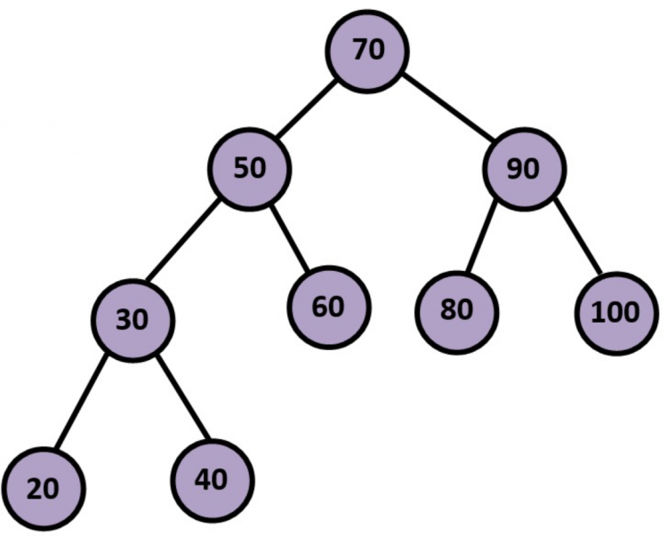
InOrder Traversal – 20 -> 30 -> 40 -> 50 -> 60 -> 70 -> 80 -> 90 -> 100
Implementation of Tree Sort Algortihm
The Tree Sort Algorithm is based on the following steps:
- Recieve an unsorted array or list as input.
- Store all the elements of the unsorted list in the binary search tree.
- Implement inorder treaversal on the binary search tree.
- Store the result of the inorder traversal into a new list and display its content.
#Creating the Queue class using linked list
class Node:
    def __init__(self, value=None):
        self.value = value
        self.next = None

    def __str__(self):
        return str(self.value)


class LinkedList:
    def __init__(self):
        self.head = None
        self.tail = None

    def __iter__(self):
        node = self.head
        while node:
            yield node
            node = node.next

class Queue:
    def __init__(self):
        self.linkedList = LinkedList()

    def __str__(self):
        values = [str(x) for x in self.linkedList]
        return ' '.join(values)

    def enqueue(self, value):
        new_node = Node(value)
        if self.linkedList.head == None:
            self.linkedList.head = new_node
            self.linkedList.tail = new_node
        else:
            self.linkedList.tail.next = new_node
            self.linkedList.tail = new_node

    def isEmpty(self):
        if self.linkedList.head == None:
            return True
        else:
            return False

    def dequeue(self):
        if self.isEmpty():
            return "The Queue is empty."
        else:
            tempNode = self.linkedList.head
            if self.linkedList.head == self.linkedList.tail:
                self.linkedList.head = None
                self.linkedList.tail = None
            else:
                self.linkedList.head = self.linkedList.head.next
            return tempNode

    def peek(self):
        if self.isEmpty():
            return "The Queue is empty."
        else:
            return self.linkedList.head

    def delete(self):
        self.linkedList.head = None
        self.linkedList.tail = None
#Creating the Binary Search Tree Class
import QueueLinkedList as queue
class BSTNode:
def __init__(self, data):
self.data = data
self.leftChild = None
self.rightChild = None#Function to insert nodes in Binary Search Tree
def insertNode(root_node, node_value):
if root_node.data == None:
root_node.data = node_value
elif node_value <= root_node.data:
if root_node.leftChild is None:
root_node.leftChild = BSTNode(node_value)
else:
insertNode(root_node.leftChild, node_value)
else:
if root_node.rightChild is None:
root_node.rightChild = BSTNode(node_value)
else:
insertNode(root_node.rightChild, node_value)
return "The node has been successfully inserted."
# Function to implement InOrder Traversal
def inOrderTraversal(root_node, tempList):
if not root_node:
return
inOrderTraversal(root_node.leftChild, tempList)
tempList.append(root_node.data)
inOrderTraversal(root_node.rightChild, tempList)#Function to implement Tree Sort Algorithm
def treeSort(tempList):
newTree = BSTNode(None)
sortedList = []
for x in tempList:
insertNode(newTree, x)
inOrderTraversal(newTree, sortedList)
print(sortedList)
unsortedList = [70, 50, 90, 30, 60, 80, 100, 20, 40]
treeSort(unsortedList)
#Output
[20, 30, 40, 50, 60, 70, 80, 90, 100]
InOrder Traversal – 20 -> 30 -> 40 -> 50 -> 60 -> 70 -> 80 -> 90 -> 100
Time and Space Complexity
The time complexity for the Tree Sort Algorithm is O(NlogN) because it takes O(logN) time to insert each element in a binary search tree and we perform this operation for all N elements. The space complexity is O(N) because we need an extra binary search tree data structure to store the unsorted data.
When to use or avoid Tree Sort
When to use Tree Sort:
- Tree Sort is useful when sorting a large number of elements.
When to avoid Tree Sort:
- The average time complexity for tree sort is O(NlogN). Hence, it can bbe avoided where time is a concern.
- The binary search tree requires higher maintenance as it needs to be re-sorted again and again.
