Pre-training
There are two types of training the BERT model
- Masked Language Model (MLM)
- Next Sentnece Prediction (NSP)
Masked Language model
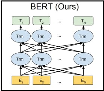
MLM is a part of the training that allows the BERT to be bidirectional compared to open IGP which used transformer but wasn’t able to use bidirectional training. MLM consists of giving BERT a sentence and optimizing the weights inside BERT to output the same sentence on the other side.
So we give the input a sentence and ask the BERT output of the same sentence but before giving sentences to the BERT we mask new tokens. We will mask the words we want to predict, so we won’t predict the whole sentence we will just pick some words in the initial sentence, apply a mask to it.
So now all the information can go in any direction without letting T2 part about the original word or any information related to it.
For example, they want to make 15% of the words replaced. In the real world use of boots, because the mask doesn’t exist in the sentences. That’s why we decided not to replace all the words with the mask always.
- Mask tokens 80% of the time.
- Sometimes replaced the original word with random tokens 10% of the time.
- Sometimes the words are left unchanged 10% of the time
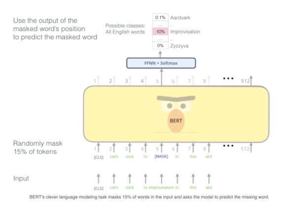
We have our inputs which are our tokenized sentences that we want to train with and in the yellow box we have the mask version of the sentence.
After the mask, we apply BERT and get vector representations for each of the inputs. BERT learns the relationship between words and the importance of context.
Now, the second training phase which is the next sentence prediction. The reason for doing this is to get a higher understanding of the language. Instead of trying just to get the meanings of the words, we actually want to get the whole meaning of sentences. Trying to get the relations between different sentences and the combined meaning of those sentences.
Convolution Neural Network (CNN) Explanation
Taking a sentence and converting it into a matrix then doing the product of matrix and feature sector will give a feature map. after completing one process we will shift the patch to one towards the right and apply exactly the same features detectors and so on.
Each time we have the highest number in the feature map that means the feature we were trying to detect is activated.
We train the matrix of feature detector in CNN, so the CNN learns to detect useful and relevant features by tunning those coefficients. Here, each feature will try to detect the relevant, valuable feature that would add information at the end of the process.
CNN Architecture
Let’s look at the different steps for architecture.
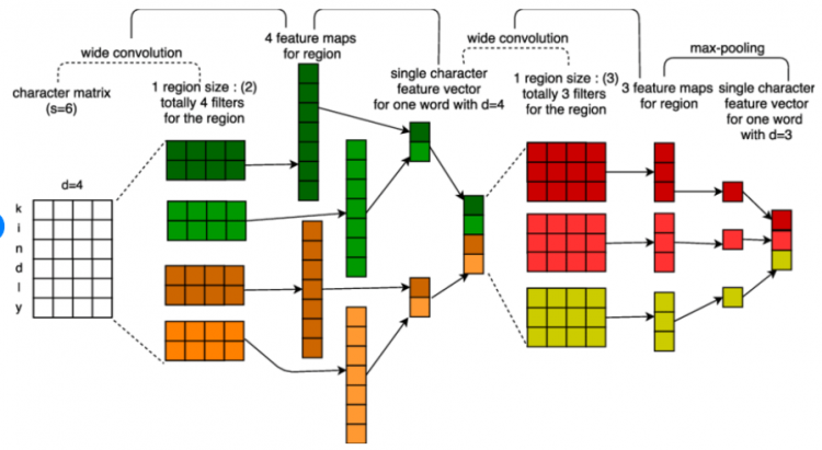
The first matrix is the input matrix having a list of words, each word being represented by a vector and how they are represented.
In the second step, we have six different feature detectors that have different sizes and they are applied to this matrix and they are applied to the first matrix.
In the third step, we have the outputs of those features detectors and the idea is that we will apply the marks to each of the third blocks. So now that all we have to do is to know whether the feature has been detected because here we have a list of all the local detections of the features that are detected by 2 blocks of feature detectors.
If we take the maximum number from the 3rd block it will tell us whether the feature is present or not in the sentence. Basically, tell us about the importance.
After that, we just need to concate all those things and apply a dense layer to get our classification tasks.
Example
Let’s take an example to understand how the BERT works. We will make a sentimental analyzer where for a given input it will give us the feeling that it conveys the meanings and gives output as a +1 if positive, 0 for negative.
The reason behind this is to extract the sentiment of the sentences using BERT.
Download the data from this website and you will have 2 CSV; train and test put those CSV into your drive folder.
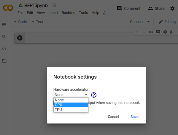
First thing is that you need to change the runtime settings of your google collab file from CPU to GPU. Went to the runtime section opt for change runtime type as given in the below picture.
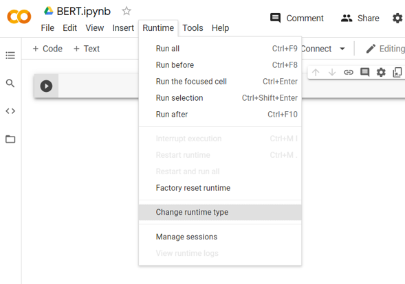
After selecting runtime type you will be having a pop-up select a GPU from there and it’s all done.
Step 1: Importing Dependencies
Importing libraries for data manipulation, ranging, and text processing too.
import numpy as np
import math
import re
import pandas as pd
from bs4 import BeautifulSoup
import random

from google.colab import drive

!pip install bert-for-tf2
!pip install sentencepiece
To make the code lighter we will import the Keras layers.
try:
  %tensorflow_version 2.x
except Exception:
  pass

import tensorflow as tf
import tensorflow_hub as hub
from tensorflow.keras import layers
import bert
Step 2: Data Preprocessing
We will import the below code, so we can have access to all the folders from our drives
drive.mount('/content/drive')After running the code you can see a link click to that link and choose your email id, then a string will appear copy-paste into this cell, and run the cell.

Enter the string in the textbox on the google colab like this

After that click on the left side panel and open the file option

After clicking on the file option you can see all the folders from your drive
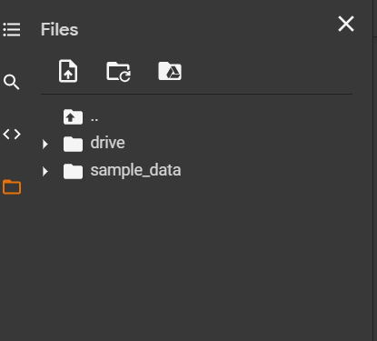
Click on the drive folder and it will show you all the files and folders from your drive.
Now we will select the path where we store our train and test file. In my case, I stored it in the BERT folder

Let’s import the data frame into the data variable and give the names of the column for the data frame.
cols = ['sentiment', 'id', 'date', 'query', 'user', 'text']
data = pd.read_csv('/content/drive/MyDrive/BERT/testdata.manual.2009.06.14.csv',
header=None,
names=cols,
engine='python',
encoding='latin1')
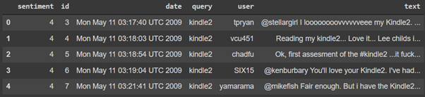
data.head()Now the data looks like this
Let’s remove some of the columns like id, date, query, and user as they are of no use right now
data.drop(['id', 'date', 'query', 'user'], axis=1, inplace=True) The data frame looks like this it’s a lighter version of the previous data frame.
data.head()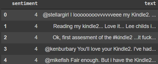
Step 3: Data Cleaning
After completing the loading process let’s clean the text.
First, let’s remove digits from the text and replace it with whitespace
tweet = re.sub(r"@[A-Za-z0-9]+", ' ', tweet)We will find the URL from the text and replace it with whitespace
tweet = re.sub(r"https?://[A-Za-z0-9./]+", ' ', tweet)We will remove the punctuations from the text and replace them with whitespace
tweet = re.sub(r"[^a-zA-Z.!?']", ' ', tweet)We will remove the extra whitespace from the text
tweet = re.sub(r" +", ' ', tweet)The full code for cleaning text, run this full code.
def clean_tweet(tweet):
  tweet = BeautifulSoup(tweet, 'lxml').get_text()
  tweet = re.sub(r"@[A-Za-z0-9]+", ' ', tweet)
  tweet = re.sub(r"https?://[A-Za-z0-9./]+", ' ', tweet)
  tweet = re.sub(r"[^a-zA-Z.!?']", ' ', tweet)
  tweet = re.sub(r" +", ' ', tweet)
  return tweet
We will keep the clean text into a data_clean
data_clean = (clean_tweet(tweet) for tweet in data.text)We will change the data_labels to 1 because our data labels are not in a sequence they are 0 for negative and 4 for positive. So we are going to change them to 0 and 1 respectively.
data_labels = data.sentiment.values
data_labels[data_labels == 4] = 1
Step 4: Tokenizing
We need to create a BERT layer to have access to metadata for the tokenizer (like vocab size). Let’s create our first BERT layer by calling hub; TensorFlow hub is where everything is stored, all the tweets and models are stored and we call from hub.KerasLayer
In the given link for the BERT model, we can see the parameters like L=12 and so on.
FullTokenizer = bert.bert_tokenization.FullTokenizer
bert_layer = hub.KerasLayer("https://tfhub.dev/tensorflow/bert_en_uncased_L-12_H-768_A-12/1",
                            trainable=False)
We will create a vocab file and store it in a variable name vocab_file
vocab_file = bert_layer.resolved_object.vocab_file.asset_path.numpy()This will tell us if we are lowercasing the text or not
do_lower_case = bert_layer.resolved_object.do_lower_case.numpy()
tokenizer = FullTokenizer(vocab_file, do_lower_case)
Let’s take an example and see if the function is working properly or not
tokenizer.tokenize('Hello, I love strawberries!')

# Output
['hello', ',', 'i', 'love', 'straw', '##berries', '!']
We saw the tokenization of sentences, let’s convert the tokens into ids.
tokenizer.convert_tokens_to_ids(tokenizer.tokenize('Hello, I love strawberries!'))

# Output
[7592, 1010, 1045, 2293, 13137, 20968, 999]
Now, we will create a function to convert all the text into the tokenized ids.
def encode_sentence(sent):
    return tokenizer.convert_tokens_to_ids(tokenizer.tokenize(sent))
Take a variable name data_inputs and now apply the cleaning functions. It will take a few seconds to run as it has a lot of weight
data_inputs = [encode_sentence(sentence) for sentence in data_clean]Step 5: Data Creation
We will create padded batches so all the sentences have the same length. That’s not a feasible option so we will group our sentences by the batch size of let’s say 32, here we will just have the first 2 sentences to have the same length inside the same batch.
By doing this, the size of the dataset will decrease and time computations for training is also taken less.
For that, we will first sort the sentence by length and store in data_with_len then apply padded_batches and then shuffle the whole data.
data_with_len = [[sent, data_labels[i], len(sent)]
                 for i, sent in enumerate(data_inputs)]
random.shuffle(data_with_len)
data_with_len.sort(key=lambda x: x[2])
sorted_all = [(sent_lab[0], sent_lab[1])
              for sent_lab in data_with_len if sent_lab[2] > 7]

all_dataset = tf.data.Dataset.from_generator(lambda: sorted_all,
                                             output_types=(tf.int32, tf.int32))
Let’s have a look at the all_dataset
next(iter(all_dataset))

# Output
(<tf.Tensor: shape=(8,), dtype=int32, numpy=array([8038, 2100, 2005, 5581, 1999, 1996, 2364, 2843], dtype=int32)>,
 <tf.Tensor: shape=(), dtype=int32, numpy=1>)
We will explicitly add the batch size and set how we want the data to look.
BATCH_SIZE = 32
all_batched = all_dataset.padded_batch(BATCH_SIZE, padded_shapes=((None, ), ()))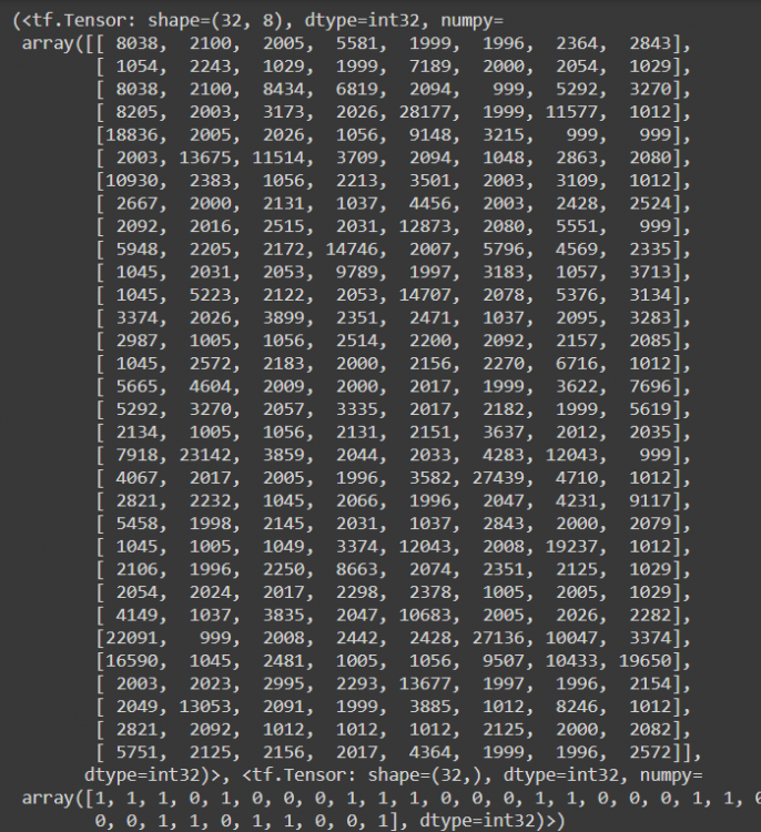
As we see in the output we have the perfect balance of 0 and 1, so we won’t have any bais.
We will get the number of batches we have right now and store them in NB_BATCHES and have test batches in NB_BATCHES_TEST which is divided by 10.
NB_BATCHES = math.ceil(len(sorted_all) / BATCH_SIZE)
NB_BATCHES_TEST = NB_BATCHES // 10
Before splitting we will shuffle all our dead sets because now we have the shortest sentences at the beginning and the longest sentences at the end.
Actually, when our dataset is not big, we can get the buffer size to be exactly the number of batches. So that’s the best way to do.
all_batched.shuffle(NB_BATCHES)
test_dataset = all_batched.take(NB_BATCHES_TEST)
train_dataset = all_batched.skip(NB_BATCHES_TEST)
Step 6: Model Building
After completing the cleaning process and data creation we will make a CNN model, let’s name the class as DCNN.
The parameters for the class will have the vocab size,
- embedding dimension we are going with the small size 128 by default,
nb_filter=50 as we give the value 50 we will have 50 feature detectors of sizes 2,3, and 4,FFN_unitswe will use the hidden units in our dense layer at the end and- giving name of the model as DCNN all keeping all the other parameters as default.
class DCNN(tf.keras.Model):

    def __init__(self,
                 vocab_size,
                 emb_dim=128,
                 nb_filters=50,
                 FFN_units=512,
                 nb_classes=2,
                 dropout_rate=0.1,
                 training=False,
                 name="dcnn"):
After initiating the class and the init function, call the super(). Now we will start creating the layers in the embedding layer.
We want vectors that are more powerful and we build those vectors with embedding layers and will be trained with the model.
 super(DCNN, self).__init__(name=name)

        self.embedding = layers.Embedding(vocab_size,
                                          emb_dim)
Let’s make convolution layers with
- the sizes of two and focus on two consecutive words and called them as bigram,
- size three and focus on three consecutive words and called them as trigram and
- size four and focus on four consecutive words and called them as fourgram.
We will keep the kernel_size as 2 for the paragraph and padding as valid; padding means sometimes sentences are so big that they will overflow the matrix so to prevent we will use valid. We will use the most commonly used activation function relu.
 self.bigram = layers.Conv1D(filters=nb_filters,
                                    kernel_size=2,
                                    padding="valid",
                                    activation="relu")
        self.trigram = layers.Conv1D(filters=nb_filters,
                                     kernel_size=3,
                                     padding="valid",
                                     activation="relu")
        self.fourgram = layers.Conv1D(filters=nb_filters,
                                      kernel_size=4,
                                      padding="valid",
                                      activation="relu")
Now we will create a layer where we will be extracting the highest value for each of those by adding a pooling layer.
self.pool = layers.GlobalMaxPool1D()Now let’s move to Feet Forward’s neural network part, we will add 2 dense layers with a hidden number of units between the two dense layers.
After adding the first dense layer we will add dropout, it is a tool that we use during training where we actually just shut down a certain number of neurons to prevent our model from overfitting.
self.dense_1 = layers.Dense(units=FFN_units, activation="relu")
self.dropout = layers.Dropout(rate=dropout_rate)
  if nb_classes == 2:
      self.last_dense = layers.Dense(units=1,
                                           activation="sigmoid")
  else:
      self.last_dense = layers.Dense(units=nb_classes,
                                           activation="softmax")
Make a class called call, the first thing we do is input the embedding layer. Let’s create the first set of outputs from the firsts et of convolutional layers. So in that way for each of our 50 features, detectors of size two, we get one number, which is maximum activation for this feature.
Now we just need to contact all the results and apply our dense layers to that
 def call(self, inputs, training):
        x = self.embedding(inputs)
        x_1 = self.bigram(x) # (batch_size, nb_filters, seq_len-1)
        x_1 = self.pool(x_1) # (batch_size, nb_filters)
        x_2 = self.trigram(x) # (batch_size, nb_filters, seq_len-2)
        x_2 = self.pool(x_2) # (batch_size, nb_filters)
        x_3 = self.fourgram(x) # (batch_size, nb_filters, seq_len-3)
        x_3 = self.pool(x_3) # (batch_size, nb_filters)

        merged = tf.concat([x_1, x_2, x_3], axis=-1) # (batch_size, 3 * nb_filters)
        merged = self.dense_1(merged)
        merged = self.dropout(merged, training)
        output = self.last_dense(merged)

        return output
The full code for training
class DCNN(tf.keras.Model):

    def __init__(self,
                 vocab_size,
                 emb_dim=128,
                 nb_filters=50,
                 FFN_units=512,
                 nb_classes=2,
                 dropout_rate=0.1,
                 training=False,
                 name="dcnn"):
        super(DCNN, self).__init__(name=name)

        self.embedding = layers.Embedding(vocab_size,
                                          emb_dim)
        self.bigram = layers.Conv1D(filters=nb_filters,
                                    kernel_size=2,
                                    padding="valid",
                                    activation="relu")
        self.trigram = layers.Conv1D(filters=nb_filters,
                                     kernel_size=3,
                                     padding="valid",
                                     activation="relu")
        self.fourgram = layers.Conv1D(filters=nb_filters,
                                      kernel_size=4,
                                      padding="valid",
                                      activation="relu")
        self.pool = layers.GlobalMaxPool1D()

        self.dense_1 = layers.Dense(units=FFN_units, activation="relu")
        self.dropout = layers.Dropout(rate=dropout_rate)
        if nb_classes == 2:
            self.last_dense = layers.Dense(units=1,
                                           activation="sigmoid")
        else:
            self.last_dense = layers.Dense(units=nb_classes,
                                           activation="softmax")

    def call(self, inputs, training):
        x = self.embedding(inputs)
        x_1 = self.bigram(x) # (batch_size, nb_filters, seq_len-1)
        x_1 = self.pool(x_1) # (batch_size, nb_filters)
        x_2 = self.trigram(x) # (batch_size, nb_filters, seq_len-2)
        x_2 = self.pool(x_2) # (batch_size, nb_filters)
        x_3 = self.fourgram(x) # (batch_size, nb_filters, seq_len-3)
        x_3 = self.pool(x_3) # (batch_size, nb_filters)

        merged = tf.concat([x_1, x_2, x_3], axis=-1) # (batch_size, 3 * nb_filters)
        merged = self.dense_1(merged)
        merged = self.dropout(merged, training)
        output = self.last_dense(merged)

        return output
Step 7: Training
Let’s set the hyper-parameters and all the information related to training.
VOCAB_SIZE = len(tokenizer.vocab)
EMB_DIM = 200
NB_FILTERS = 100
FFN_UNITS = 256
NB_CLASSES = 2

DROPOUT_RATE = 0.2

NB_EPOCHS = 5
Let’s give all the parameter values.
Dcnn = DCNN(vocab_size=VOCAB_SIZE,
            emb_dim=EMB_DIM,
            nb_filters=NB_FILTERS,
            FFN_units=FFN_UNITS,
            nb_classes=NB_CLASSES,
            dropout_rate=DROPOUT_RATE)
Now we need to combine and give it to the optimizer and loss function and find accuracy.
if NB_CLASSES == 2:
    Dcnn.compile(loss="binary_crossentropy",
                 optimizer="adam",
                 metrics=["accuracy"])
else:
    Dcnn.compile(loss="sparse_categorical_crossentropy",
                 optimizer="adam",
                 metrics=["sparse_categorical_accuracy"])
We will create a checkpoint list in the drive. We will need a checkpoint because after the training is done we want to get back the weights that have been trained and to use them later.
checkpoint_path = "./drive/MyDrive/projects/BERT/ckpt_bert_tok/"

ckpt = tf.train.Checkpoint(Dcnn=Dcnn)

ckpt_manager = tf.train.CheckpointManager(ckpt, checkpoint_path, max_to_keep=1)

if ckpt_manager.latest_checkpoint:
    ckpt.restore(ckpt_manager.latest_checkpoint)
    print("Latest Checkpoint restored!")
We will make a custom class which we will give to the fit functions so that it executes any lines of codes between each epoch or between its patch.
class MyCustomCallback(tf.keras.callbacks.Callback):

    def on_epoch_end(self, epoch, logs=None):
        ckpt_manager.save()
        print("Checkpoint saved at {}.".format(checkpoint_path))
Now we will use a callback for our fit method.
Dcnn.fit(train_dataset,
         epochs=NB_EPOCHS,
         callbacks=[MyCustomCallback()])
Step 8: Evaluation
Let’s see the results, by running the below code.
results = Dcnn.evaluate(test_dataset)
print(results)
We will make a prediction function where we will input the sentence and we will get an output as negative or positive.
def get_prediction(sentence):
    tokens = encode_sentence(sentence)
    inputs = tf.expand_dims(tokens, 0)

    output = Dcnn(inputs, training=False)

    sentiment = math.floor(output*2)

    if sentiment == 0:
        print("Output of the model: {}\nPredicted sentiment: negative.".format(
            output))
    elif sentiment == 1:
        print("Output of the model: {}\nPredicted sentiment: positive.".format(
            output))
Let’s call the function with an input sentence.
get_prediction("This movie was pretty interesting.")

# Output
Output of the model: [[0.95817465]]
Predicted sentiment: positive.