In the previous article, we explored the Naive Bayes algorithm for an NLP task. In this article, we look at another popular ML algorithm for NLP called the Support Vector Machines or SVM algorithm. We will also perform sentiment analysis using the same.
The SVM algorithm
The SVM or Support Vector Machines algorithm just like the Naive Bayes algorithm can be used for classification purposes. So, we use SVM to mainly classify data but we can also use it for regression. It is a fast and dependable algorithm and works well with fewer data.
A very simple definition would be that SVM is a supervised algorithm that classifies or separates data using hyperplanes. So, this algorithm is a supervised algorithm in which we pass the data as well as the labels of the classes to the model. We pass the data and its corresponding label.
But what are hyperplanes?
Let’s look at the following image. In the image, we recognize that there are two groups or classes of points. One class is the black points and another one is the blue points. What can we do to make the distinction between them visible?
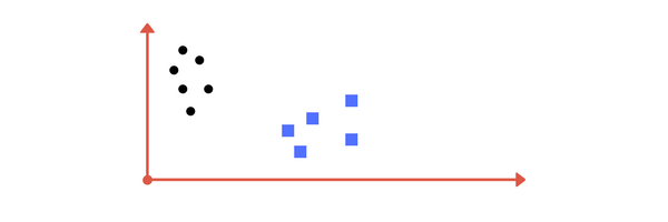
We could draw a line between them. That would separate them perfectly. The line that separates them is called the decision boundary or hyperplane (in 2D). Notice that the points are in 2-dimensions as we can only see two axes i.e. the x and y-axis. Hence, here the hyperplane is a line.
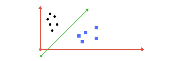
Remember, just like a line separates data in 2-D so does a hyperplane in multidimensional space. So a hyperplane as the name suggests is a plane in n-dimensional space that separates classes or groups of data. In 2-D the hyperplane can be seen as a line but in higher dimensions, it’s could be very complex.
Just so that we are on the same page, we have seen that the SVM algorithm has the job of separating groups of data by fitting a hyperplane. We have also seen that in 2-dimensional space, the hyperplane is a line that separates the groups but as the dimensions increase the hyperplane acts like a complex plane to separate groups of data.
How do we separate non-linear data?
In the previous section and images, the data we had seen was linearly separable i.e the data could be separated by just drawing a straight line between the classes. But look at the following image.
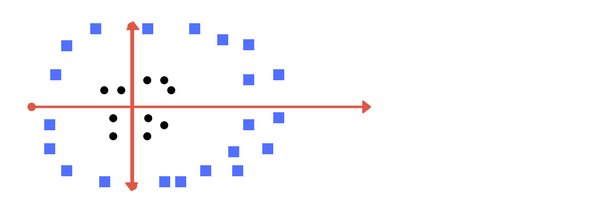
The data points in the image above cannot be separated by a straight line to separate the blue and black points. So how will the SVM algorithm be able to fit an optimal hyperplane that separates both the classes in the data? In this case, the algorithm will map these points to a higher dimension.
Since the data was inseparable in 2-D, the algorithm added another dimension to it. So now our data is in a 3-dimensional space and it looks like in the image shown below. To get a better understanding of the image, think of the previous image as the top view and the following image as the side view with an added dimension.
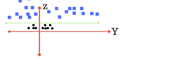
By adding a new dimension, we can view the data w.r.t to the z-axis. Now, the data is linearly separable from this perspective and the algorithm fits a hyperplane to separate the data. Let’s assume that the mapping on the z-plane follows the formula w = x^2 + y^2. After separation, we return to the lower dimension. The data looks like this now.
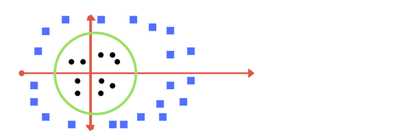
It would be easier to understand this view as the top view (2-D) after returning from the side view (3-D) because now we cannot see the z-axis, only x and y coordinates. What seemed like a line in 3-D is actually a circle in 2-D. The data is now separated.
The “optimal” hyperplane
We have seen how the algorithm separates different datasets to classify them correctly. It maps the data to a higher-dimensional space if the data is not separable in the lower dimensions. The algorithm doesn’t just fit any hyperplane, it tries to fit an optimal hyperplane.
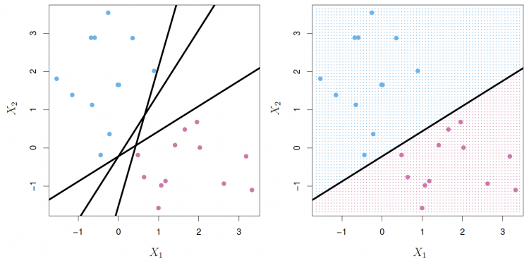
As shown in the images above, we have blue and red data points. We want the SVM algorithm to separate them so that it can learn and classify new unseen points as red or blue. As seen in the left image, the SVM algorithm can pick any of the shown hyperplanes (again, remember, we are in 2-D so hyperplane is a line) as all of the hyperplanes separate the points.
But the algorithm picks a hyperplane like the one shown in the right image. If you look at the hyperplane chosen by the model and the available options, you will see that the hyperplane on the right separates the data points well which will help the model to generalize better on unseen data points.
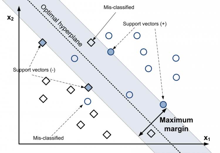
To know how the model chooses this optimal hyperplane, we have to focus on the above image. As you can see the optimal hyperplane is shown by the dotted line. The data points at the forefront of a class closest to the opposite class are called support vectors.
As you can see, support vectors are marked in the image. These support vectors are the points of a class closest to the separating boundary i.e points of a class closest to the opposing class. So, the model will try to fit a hyperplane that maximizes the distance between these support vectors. This is the optimal hyperplane.
The optimal hyperplane in the image is shown to be at such a position that the distance between the support vectors of both classes is maximum. This is called the maximum margin and is labeled in the image.
Doing sentiment analysis using SVM
Sentiment analysis is finding the polarity of a document. It is a type of algorithm that helps us judge the tone of a document, i.e. whether it is positive, negative, or neutral. Sentiment analysis is also called opinion mining or polarity detection.
For example, if we have a business and are interested in knowing how customers feel about a certain product or campaign, we can access the related Twitter data and with the help of sentiment analysis tools, we can see if a majority of the tweets are positive, negative or neutral.
There is no doubt that sentiment analysis is gaining popularity in the industry as it allows organizations to mine the opinions of a large group of users or potential customers in a cost-efficient way, just as we had discussed above.
To build a sentiment analysis tool we will be using the same dataset we had used for building the model using the Naive Bayes algorithm in the previous post. If you also want to know how we built the sentiment analysis model using Naive Bayes then refer to our post on the Naive Bayes algorithm.
The dataset we will be using to build a sentiment analyzer can be found at http://archive.ics.uci.edu/ml/datasets/Sentiment+Labelled+Sentences. Once on the webpage, click the download data folder and download the zip file. After the download is complete, extract the files and you are good to go.
We will begin by importing the necessary modules and packages.
import pandas as pd
from sklearn.feature_extraction.text import CountVectorizer
from sklearn.feature_extraction.text import TfidfTransformer
from sklearn.model_selection import train_test_split
from sklearn.svm import SVC
from sklearn.metrics import confusion_matrix
import numpy as np
If you are working in Google colab then you can mount your drive using the code given below. Upload the downloaded data to your drive and set the correct path to use the data.
from google.colab import drive
drive.mount('/content/drive')
Now, set the correct path to where you have uploaded the data in your Google drive.
dataset_path = "/content/drive/MyDrive/Datasets/amazon_cells_labelled.txt"We now read the dataset using the pandas read_csv function. This function helps us to read data efficiently from a CSV file into a dataframe. We are using the tab as a separator and we do not set a header. Run the code below to achieve this.
data = pd.read_csv(dataset_path, sep="\t", header=None)Now that we have loaded the dataset, we check the first 10 rows using the head method.
data.head(10)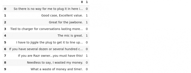
This is the data we will be working with. As you can see it consists of customer reviews and the corresponding labels. The labels are either 0 (indicating a negative sentiment) or 1 (indicating a positive sentiment).
We now want to separate the text and the labels so that we can work with the text easily and get it ready for modeling. Use the code below to extract the text.
X = data.iloc[:,0]
X

# Output:
0      So there is no way for me to plug it in here i...
1                            Good case, Excellent value.
2                                 Great for the jawbone.
3      Tied to charger for conversations lasting more...
4                                      The mic is great.
                             ...
All the reviews are now assigned to the variable X. Now we extract the sentiment labels and assign them to the variable y.
y = data.iloc[:,-1]
y

# Output:
0      0
1      1
2      1
3      0
4      1
      ..
Now that we have segregated text and sentiments, we will prepare the text for further tasks.
We will vectorize the text using the count vectorizer. We also filter the stopwords in this step by passing the stop_words parameter. We then fit this vectorizer onto our text data.
vectorizer = CountVectorizer(stop_words='english')
X_vec = vectorizer.fit_transform(X)
After running the above step, we get a sparse matrix which is the result of applying the sparse matrix to our dataset. We now convert it into a dense matrix and check it out.
X_vec = X_vec.todense()
X_vec

# Output:
matrix([[0, 0, 0, ..., 0, 0, 0],
        [0, 0, 0, ..., 0, 0, 0],
        [0, 0, 0, ..., 0, 0, 0],
        ...,
        [0, 0, 0, ..., 0, 0, 0],
        [0, 0, 0, ..., 0, 0, 0],
        [0, 0, 0, ..., 0, 0, 0]])
We now apply TF-IDF transformation to the data. Note that we are applying TF-IDF transformation to the Bag of Words model we created in the previous step. We would get a better representation of the data.+
tfidf = TfidfTransformer() # by default applies "l2" normalization
X_tfidf = tfidf.fit_transform(X_vec)
X_tfidf = X_tfidf.todense()
X_tfidf

# Output:
matrix([[0., 0., 0., ..., 0., 0., 0.],
        [0., 0., 0., ..., 0., 0., 0.],
        [0., 0., 0., ..., 0., 0., 0.],
        ...,
        [0., 0., 0., ..., 0., 0., 0.],
        [0., 0., 0., ..., 0., 0., 0.],
        [0., 0., 0., ..., 0., 0., 0.]])
Now, our text data is converted into a matrix of TF-IDF representation.
After this, we need to split the dataset into train and test sets. We do this because we want to evaluate the performance of our trained model. Remember that we first train the model i.e. let it learn on the training set and then we test it on an unseen dataset i.e. the test dataset. This is called cross-validation.
To split the data we use the train_test_split function. We set the test_size to equals 0.25 indicating that 75% of the data will be split for training and 25% for testing.
X_train, X_test, y_train, y_test = train_test_split(X_tfidf, y,
                                                    test_size = 0.25,
                                                    random_state = 0)
We now instantiate the SVM model and fit the model on the training dataset. This is where our model learns.
We use the linear kernel to separate our data linearly. Another popular kernel is the RBF kernel.
classifier = SVC(kernel='linear')
classifier.fit(X_train, y_train)
After the model is trained, we use it to predict the sentiments of data that is unseen by the model i.e. the test data. We save these predicted values in y_pred.
y_pred = classifier.predict(X_test)We can judge the performance of our model by computing the confusion matrix. This matrix is an indicator of how well the model performed on this task of sentiment analysis. Basically, we are comparing the predicted and actual or true values.
confusion_matrix(y_test, y_pred)

# Output:
array([[102,  18],
       [ 33,  97]])
For the scikit-learns confusion matrix,
- The values in vertical axis represent the actual values
- The values in horizontal axis represent the predicted values
- The total number of correct predictions are obtained by summing the left diagonal.
So, our model predicted 135 (102 + 33) values as having a negative sentiment (0) out of which 102 were correctly predicted and 33 were incorrectly predicted. Our model also predicted 115 (18 + 97) values as having a positive sentiment (1) out of which 97 were correctly predicted and 18 were incorrectly predicted.
The total number of correct predictions can be obtained from the confusion matrix by summing the left diagonal. In this confusion matrix, we get the total correct predictions of 199 (102 + 97). We can also calculate the accuracy of our model by using the confusion matrix.
To calculate the accuracy of the model we need to divide the total correct predictions by the total count of the test set (summing all the numbers in the confusion matrix). So the accuracy of our model is 199/250 = 79.6%
If we compare it with the Naive Bayes model, then SVM performed slightly better than Naive Bayes.
The complete code used in this article is given below for quick reference.
import pandas as pd
from sklearn.feature_extraction.text import CountVectorizer
from sklearn.feature_extraction.text import TfidfTransformer
from sklearn.model_selection import train_test_split
from sklearn.svm import SVC
from sklearn.metrics import confusion_matrix

from google.colab import drive
drive.mount('/content/drive')

dataset_path = "/content/drive/MyDrive/Datasets/amazon_cells_labelled.txt"
data = pd.read_csv(dataset_path, sep="\t", header=None)
data.head(10)

X = data.iloc[:,0]
X

y = data.iloc[:,-1]
y

vectorizer = CountVectorizer(stop_words='english')
X_vec = vectorizer.fit_transform(X)
X_vec = X_vec.todense()
X_vec

tfidf = TfidfTransformer() # by default applies "l2" normalization
X_tfidf = tfidf.fit_transform(X_vec)
X_tfidf = X_tfidf.todense()
X_tfidf

X_train, X_test, y_train, y_test = train_test_split(X_tfidf, y,
                                                    test_size = 0.25,
                                                    random_state = 0)

classifier = SVC(kernel='linear')
classifier.fit(X_train, y_train)

y_pred = classifier.predict(X_test)

confusion_matrix(y_test, y_pred)
Final thoughts
In this article, we have been introduced to the SVM algorithm, we have also looked at the working of the algorithm and finally, we built a sentiment analysis tool using the SVM algorithm which performed marginally better than other models by giving a good accuracy score.
Thanks for reading.