Working with Multiple DataFrames in Pandas

We will take a deeper dive into the mechanics of working with multiple datasets. When working with data to address specific analytical questions we often need to combine multiple DataFrames.

We are going to familiarize ourselves with the mechanics of combining or concatenating datasets, with the primary focus on the structural aspect of the operation. We will also be discussing the more advanced operations like joins, cardinality, inner, outer, left, and right joins.

We are going to use five datasets containing the salary information for US colleges by region and major. The dataset we’ll be exploring comes from a number of sources including the Kaggle Wallstreet Journal.

Concatenating DataFrames

To concatenate two or more DataFrames we use the Pandas concat method. The method helps in concatenating Pandas objects along a particular axis.

We have five DataFrames that look structurally similar but are fragmented. Let us check the shape of each DataFrame by putting them together in a list.

# Storing the DataFrames in a list
dfs = [state, eng, liberal, ivies, party]

for df in dfs:
    print(df.shape)

# Output:
(175, 4)
(19, 4)
(47, 4)
(8, 4)
(20, 4)

We see that all the DataFrames have different numbers of schools, which is why their indices are of different lengths but they all have four columns.

Now, for example, let us say we wish to concatenate two DataFrames, the Engineering Schools with the Ivy League Schools.

pd.concat([ivies, eng])

We get a new DataFrame which is the combination of the Ivy League Schools and the Engineering Schools. Now when we check the shape of the new DataFrame, we see that it is consistent with the sum of the lengths of the two DataFrames respectively.

# Shape of the new concatenated DataFrame
pd.concat([ivies, eng]).shape

# Output
(27, 4)

# Sum of the shape of individual DataFrames
ivies.shape[0] + eng.shape[0] 

# Output
27 

NOTE: If we wish to concatenate multiple DataFrames together, we can simply pass on a list of all the DataFrames to the concat function.

pd.concat([state, eng, liberal, ivies, party])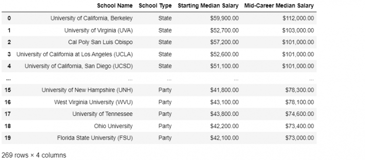

The Duplicated Index Issue

The DataFrame we created by concatenation had a lot of duplicate indices. For example, if we run the loc indexer for any index value, we may get more than one associated row.

schools.loc[0]

As we can see in the result of the above command, there is more than one row associated with the index ‘0’. This happens because each DataFrame that we concatenated had its own index value ‘0’. Thus, each of these values is reflected in the search results, giving rise to duplicacy.

All this happens because the concat method does not discard the original index of the DataFrame being concatenated.

However, in Pandas, it is not technically invalid to have duplicated values for the indices. Nothing breaks if duplicate indices exist in a DataFrame. But the problem is that multiple functionalities stop working.

Another problem is that when the indices do not contain unique values, slices no longer work. Thus, it is good practice to remove duplicate indices because the data becomes misleading if they are not.

For instance, we will run the following code to slice some of the indices.

schools.loc[0:2]

The DataFrame does not hold unique values for indices. Hence, we receive the error “Cannot get slice bound for the non-unique label” because the function cannot make use of a non-unique label.

For these reasons, the preference when combining DataFrames is to have at least one common index with unique values across all records. This can be achieved by using any of the ways mentioned below.

Reset Index on the DataFrame

We use the reset_index method to reset the indices of the DataFrame. It restores a zero-based range index in a DataFrame while relegating the old index to a new column in the resulting DataFrame.

However, we don’t need the newly created column for any functionality. Hence, we will go ahead and set the drop parameter of the reset_index method to True. Now, the following command will reset the duplicate indices without assigning them a new column.

schools.reset_index(drop = True, inplace = True)

We can confirm whether or not the newly created DataFrame has unique indices by using the duplicated function.

schools.index.duplicated()

# Output
array([False, False, False, False, False, False, False, False, False,
       False, False, False, False, False, False, False, False, False,
       ...,
       False, False, False, False, False, False, False, False, False,
       False, False, False, False, False, False, False, False])
​

Discard Old Index during Concatenation

A more elegant approach to avoid the creation of duplicate indices is to discard them at the time of concatenation. This way, we do not need to practice cleanup later.

Hence, we can modify the concat function in the following manner:

pd.concat(dfs, ignore_index = True).drop_duplicates(subset = ['School Name'])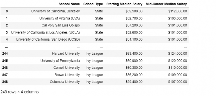

The ignore_index parameter, when set to True, ignores the old indices of the concatenated DataFrames and creates a new column with unique indices.

By using this method, we ensure that there are no overheads after the DataFrames have been concatenated. It is more time-efficient as it discards duplicate indices at the same time as concatenation.

Enforcing Unique Indices

We have dealt with the problem of duplicated indices by resetting the DataFrame index or by completely ignoring the duplicates during concatenation. These options might be inadequate for some cases. For example, when we want to preserve the index and force uniqueness.

For this, the concat function has a parameter as verify_integrity which helps in ensuring unique indices. This parameter when set to True, Pandas will throw an error when it encounters a duplicate index.

For example, we set the School Name as the index for the Ivy League and Engineering Schools. We add a random sample from the Engineering Schools to the Ivy League DataFrame and run the concat function with verify_integrity set to True.

ivies2 = ivies.set_index('School Name')
eng2 = eng.set_index('School Name')

ivies2 = ivies2.append(eng2.sample())

pd.concat([ivies2, eng2], verify_integrity = True)

we receive the error “Indices have overlapping values”. In order to remove this error, we have two options:

• OPTION 1: We could choose a different index for the DataFrames we are concatenating, something other than the School Name in this case.
• OPTION 2: We could even relax this condition by setting the verify_integrity back to the default state, i.e. False and deal with the duplicates otherwise, for example by resetting the index and regenerating the index.

Column Axis Concatenation

Till now we have only used the concat method to combine the DataFrames along the row axis, and we ended up with a single long DataFrame.

If we wish to change this behavior and want to concatenate along the column axis, we only need to modify the axis parameter, from the default of 0 to 1, in the concat method.

Let us say, we want to reflect the top 5 Ivy League and Engineering Schools that produce the highest-earning graduates.

• STEP 1: We start by creating sorted copies of our DataFrames in Descending order, drop the original indices, then selecting the top 5 and finally, storing them in seperate variables.

# Sorting the ivies DataFrame in descending order by Median Salary
ivies3 = ivies.sort_values(by = ['Starting Median Salary'], ascending = False)[:5]
                  .reset_index(drop = True)

# Sorting the eng DataFrame in descending order by Median Salary
eng3 = eng.sort_values(by = ['Starting Median Salary'], ascending = False)[:5]
                  .reset_index(drop = True)

• STEP 2: Now that we have the required DataFrames displaying the top 5 schools. We need to put them side-by-side horizontally in a new DataFrame.

# Concatenating along the column axis
pd.concat([ivies3, eng3], axis = 1)

The append Method

The append and concat method are quite similar to each other. The append function adds a new item to the end of the list, which means that it simply modifies the existing DataFrame.

For example, we wish to add the Liberal Schools to the Party Schools using both the append and concat methods.

• Using the append method.

# Adding party to liberal using append method
liberal.append(party)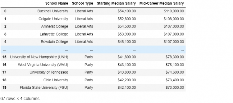

• Using the concat method.

# Adding party to liberal using concat method
pd.concat([liberal, party])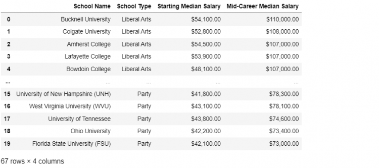

In this particular use case, there is no difference between the outputs of the two methods but there are a couple of differences in how they behave.

• The append method is an instance method and it can only be called on existing DataFrames and Series objects. The concat method, on the other hand, is called directly from the imported Pandas module.
• The concat method is a lot more flexible since it gives us the flexiblilty to concatenate along the column as well as the row axis. The append method doesn’t concatenate along the columns and its axis parameter is fixed to 0.

We can think of append as a special case of concat where the axis is fixed to 0.

Using concat on Different Columns

So far, we have only worked with DataFrames that stack up perfectly. This means that they have the same number of columns with the same names. Hence, we have had no problems while performing concatenation.

Sometimes, this will not be the case. For example, if we have to concatenate a DataFrame with another one having an extra column that is not required, we would need to apply a different approach.

To implement this example, we will create an additional column “STEM” which stands for “Science Technology Engineering Mathematics”.

• STEP 1: Firstly, we will create a copy of the eng DataFrame because we don’t want the changes to be reflected in the original data.

eng4 = eng.copy()

• STEP 2: We will add the “STEM” column and initiate it to True. Then, we can use the head to check whether the column has been successfully added.

eng4['STEM'] = True
eng4.head()

• STEP 3: Now, we need to concatenate the modified DataFrame with the ivies DataFrame.

pd.concat([ivies, eng4])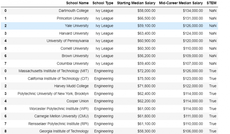

As we can see, the “STEM” column has been included in the resultant DataFrame. The column has “NaN” value as the default for all elements that are in the ivies DataFrame and does not have this column initially.

However, if we set the join parameter of concat to inner instead of outer, we are indicating that we require only those columns which are common to both the DataFrames. In the following example, the “STEM” column will not appear in the resultant DataFrame.

pd.concat([ivies, eng4], join = 'inner')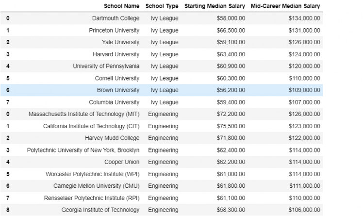

The merge Method

The merge method allows us to combine DataFrames using techniques and logic very similar to the Structured Query Language (SQL). The merge function gives us a flexible interface to join various DataFrames and objects.

How is joining or merging different from concat

The concat or the related append method is an operation that glues together pieces of data into one unified data structure. It is a structure-focused operation.

The merge method on the other hand gives us a lot more options to flexibly combine multiple datasets on the basis of content they have in common. The merge method is a content-based operation.

Let us understand this using an example, suppose we need to extend our schools DataFrame, which was a concatenation of all the schools in a single DataFrame, with the additional information from a new regions DataFrame.

pd.merge(schools, regions)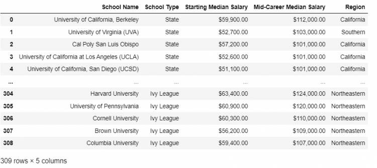

The merging automatically happens by the School Name, which happens to be the only column common in both the DataFrames. This behavior is controlled by the on parameter in the merge function. Therefore, the code is equivalent to:

pd.merge(schools, regions, on = 'School Name')

The left_on and right_on parameters

Very often we come across DataFrames we want to merge but do not have a key column of the same name.

Let us suppose, we wish to extend our existing schools DataFrame with the help of a new dataset mid_career that provides us the mid-career percentile salary of graduates from each school.

The key columns are clearly the school names but even though the key columns are consistent datasets, they both are named something else. The schools DataFrame has the school name column as School Name and the mid_career DataFrame has the column as school_name.

Now, if we perform the merge function without any parameters we get an error saying “No common columns to perform merge on” because the Pandas doesn’t know exactly what to merge on.

To fix this, we have the left_on and right_on parameters which contain the key columns in each DataFrame.

pd.merge(schools, mid_career, left_on = 'School Name', right_on = 'school_name')

Consider the merge function to always be operating on two objects, one on the left and the other on the right. Using the left_on and right_on parameters we specify exactly what the key column from each object should be.

We also notice that the resultant DataFrame has an extra school_name column which adds to the redundancy of the output since it is not adding on to any information. To remove this we append the drop method and remove the school_name column.

pd.merge(schools, mid_career, left_on = 'School Name', 
         right_on = 'school_name').drop('school_name', axis = 1)

Inner and Outer Joins

We have used the merge method to join separate DataFrames by relying on a column they have in common called the Key Column. Now we will be discussing what logic should apply while merging the two datasets.

The type of join operation in Pandas is controlled by the how parameter in the merge method. The terminologies are quite similar to Structured Query Language (SQL).

The Inner Join

The inner join only returns the records that are present on both right and left objects. The merge function by default performs an inner join on the given two DataFrames.

Let us take an example that we want to merge the ivies DataFrame with the regions information we have available.

pd.merge(ivies, regions, how = 'inner')

The inner join returns the elements common to both DataFrames and in this case only the Ivy League Schools which show up in both regions and the ivies DataFrame.

Only the common keys are selected, which means the inner join gives us the intersection of the two DataFrames.

The Outer Join

The outer join returns the records which are present in either the left or right of the two DataFrames. We can think of the outer join as making sure that all the records from both DataFrames are reflected in the resulting merge.

pd.merge(ivies, regions, how = 'outer')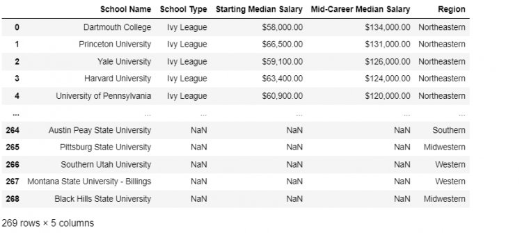

Outer joins are like Union since we are combining a set of keys from the left DataFrame and the set of keys from the right DataFrame using a union operation.

Left and Right Joins

The merge method also supports two other join methods, specifically the Left Join and the Right Join. These are comparatively easier than the Inner and Outer Joins.

The type of join operation in Pandas is controlled by the how parameter in the merge method.

The Left Join

When doing a left join, we are specifying that we want to preserve the key indices on the left object, merge the data, and discard everything else.

Let us merge the ivies and the regions DataFrame using the Left Join.

pd.merge(ivies, regions, how = 'left')

In this case, we have kept all the Ivy League Schools, added the Region column for all of them, and discarded all the other keys from the right DataFrame.

The Right Join

The Right Joins are just the opposite of the Left Join operation. If we change the how parameter to right, we now tell Pandas to preserve all the unique keys on the right object, join the two objects, and discard everything else.

pd.merge(ivies, regions, how = 'right')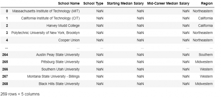

One-to-One and One-to-Many Joins

When combining multiple datasets or tables, we are going to come across terminology that describes the type of association between different elements in our data.

One-to-One Joins

A one-to-one join happens when each record in a DataFrame is associated with one record in another dataset.

Let us check out the ivies DataFrame, we see a list of eight unique universities.

And let us pick up the regions DataFrame for reference.

Let us merge ivies with regions using the default parameters.

pd.merge(ivies, regions)

Now the question arises if is this a one-to-one join. To determine whether each Ivy League School in the ivies DataFrame is associated with one and only one record on the regions DataFrame.

The answer comes down to whether the two datasets both have unique values in the resulting key column. In our case, the key column is the School Name. For the ivies DataFrame we clearly see that the School Name contains unique values.

To find out the uniqueness of the regions DataFrame, since we cannot visually confirm, we will take a different approach here. We will isolate the records for the School Names containing the ivies DataFrame.

regions[regions['School Name'].isin(ivies['School Name'])]

Here, we have created a boolean mask that checks whether each school in regions is in ivies, and then the square brackets select only the True elements from the regions dataset.

We get back exactly the eight Ivy League Schools, so we have confirmed that both the datasets have unique values on the key column for the keys they have in common. Therefore, the type of join we have is a One-to-One Join.

One-to-Many Join

One-to-many relationships associate one record in one DataFrame with many records in the other DataFrame.

Let us take another look at another set of schools, namely the state schools and we wish to merge this dataset with the regions DataFrame. We end up with the question that which kind of a join will we end up using in this situation.

The answer depends upon whether we have duplicates in our respective key columns or the keys selected by the inner join operation. Now we need to check whether the state dataset contains only unique school names.

state['School Name'].is_unique

# Output
True

The is_unique attribute indicates that the school names contained in the state DataFrame is unique. Now, let us check the regions DataFrame for the same.

regions['School Name'].is_unique

# Output
False

Using the following command, we can check if there are some schools that show up more than once.

regions[regions['School Name'].isin(state['School Name'])]
        .loc[:, 'School Name'].value_counts()

# Output
University of New Hampshire (UNH)                     2
Florida State University (FSU)                        2
University of Florida (UF)                            2
...
University of California, San Diego (UCSD)            1
Name: School Name, Length: 175, dtype: int64

So, we have confirmed that the regions DataFrame does not have unique school names. If we go ahead and perform the merge operation, we will be looking at a one-to-many association.

pd.merge(state, regions, on = 'School Name', how = 'inner')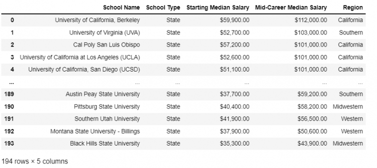

This kind of merge is one-to-many because the left object has unique key column values whereas the right column duplicates some of them. The merged DataFrame for one-to-many associations will duplicate the records that appear more than once.

NOTE: If we wish to remove the duplicate values from the resulting DataFrame in a one-to-many join, we can use the drop_duplicates method to do so. We can either remove the duplicates first, and perform a one-to-one join, or perform a one-to-many join and remove the duplicates afterward.

Many-to-Many Join

Many-to-Many Joins occur when we have duplicates in the key columns from both left and right objects that are being merged.

Let us create a new survey DataFrame where we assume we asked four people about the prestige value an Ivy League or an Engineering degree has.

survey = pd.DataFrame({
    'School Type': ['Ivy League', 'Ivy League', 'Engineering', 'Engineering'],
    'Prestige': ['High', 'Good', 'Good', 'Okay'],
    'Respondents': [1, 2, 3, 4]
})

Now, we wish to merge this survey data with the ivies DataFrame. The key column, in this case, is the School Type.

We notice that the School Type column in both the DataFrame objects contains duplicates and when we merge these two DataFrames, we get a many-to-many association.

pd.merge(ivies, survey)

The resultant DataFrame has twice the number of records. Each School has been duplicated to make room for the variability in the survey data.

Merging by Index

Occasionally we might be interested in joining by index instead of columns, fortunately, the Pandas’ merge method fully supports that.

Let us set the School Name as the index of the two DataFrames ivies and regions and store them in separate variables.

ivies4 = ivies.set_index('School Name')

regions2 = regions.set_index('School Name')

Now if we try to merge the two DataFrames, the Pandas will rightly throw an error that it has “No common columns to perform the merge on“.

pd.merge(ivies4, regions2)

We need a way to tell Pandas that we need to do the merge using the index axis as the key column. To do that we use the left_index and right_index parameters to indicate we need the respective indices to act as the key columns for the merge.

pd.merge(ivies4, regions2, left_index = True, right_index = True)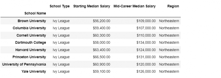

Merging by index and columns

One interesting combination that arises is if we want to merge using the index on one DataFrame and a column on the other. That could be easily done by combining the right_index by left_on or right_on by left_index.

Let us merge ivies4, which has School Name as the index, with regions having a range index.

pd.merge(ivies4, regions, left_index = True, right_on = 'School Name')

The join Method

For the types of joins, specifically index-on-index and columns-on-index, Pandas provide a convenient DataFrame method called join.

ivies4.join(regions2)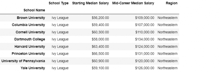

This is a shorter call as compared to the merge operation. The join operation can also merge DataFrame using any of its columns as key and matching it on another DataFrame’s index.

Let us merge regions2, which has School Name as the index, with ivies having a range index.

ivies.join(regions2, on = 'School Name')