We will be taking a closer look into the advanced Pandas indexing feature, the MultiIndex. We are going to build an understanding of modifying the axis, primarily the index, in order to support more than one level of labels. This allows us to reflect multi-dimensional datasets.
We will be working with hierarchical indices, techniques, and methods like slicing, sorting, swapping, shuffling, and pivoting index levels.
Introducing New DataFrames
We are going to explore a new dataset that contains daily stock price information on NASDAQ for the past five and a half years for five of the largest US technology companies, namely Apple, Facebook, Microsoft, Google, and Amazon.
Importing the DataFrame:
import numpy as np
import pandas as pd
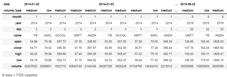
tech = df = pd.read_csv("C:/Users/BHAVYA/Documents/tech_giants.csv")
tech.head()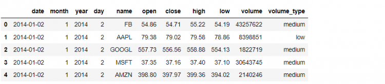
To calculate for how many years the data has been recorded, we can use the following approach:
tech.year.value_counts()/5

# Output
2016    252.0
2014    252.0
2015    252.0
2017    251.0
2018    251.0
2019    163.0
Name: year, dtype: float64
Let us now set the index of the DataFrame from a range index to something more meaningful such as the date.
# Setting date as the Index
tech.set_index('date')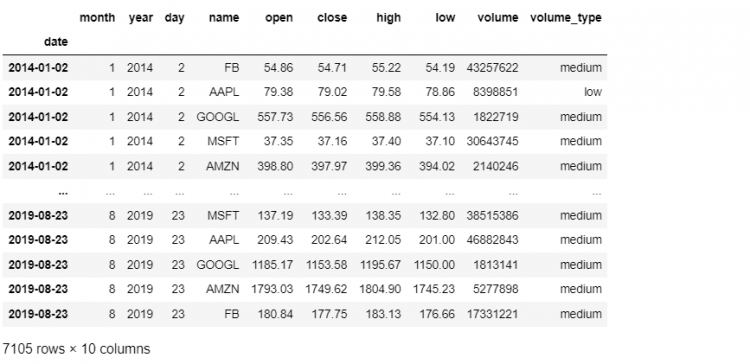
Creating a Multi-Index
We use a multi-index when we need more than one field index for our DataFrame. A multi-index is also called a Hierarchical Index. Using a multi-index we create a hierarchy of indices within the data.
So, instead of date, we will pass in a list of strings. This will indicate to Pandas that we want all the column names to act as the index for our DataFrame.
tech.set_index(['date', 'name'], inplace = True)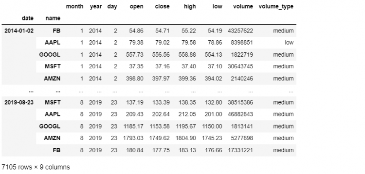
The resultant DataFrame is a multi-index. It means that a single index object has more than one level or component to it. When we promoted the date and name columns as the index, they were removed from our DataFrame and they no longer show up as regular columns.
type(tech.index)

# Output
pandas.core.indexes.multi.MultiIndex
Multi-Index from read_csv Method
Previously, we had created a multi-index from our technology stocks dataset by first, reading in the data and then, using the set_index method to specify date and name as the two levels of our multi-index.
Now, we will be looking at an alternative way to arrive at the same DataFrame, but in a single step.
Let us use the read_csv method to read the data again, but this time we will rely on the index_col parameter in the read_csv method to indicate that we want a multi-index in the resulting DataFrame.
tech = pd.read_csv("C:/Users/Documents/tech_giants.csv", index_col = ['date', 'name'])Another approach to creating a multi-index DataFrame would be to create a multi-index object separately and then pass it to the Pandas DataFrame constructor.
pd.DataFrame(data, index = MultiIndexObject)Indexing Hierarchical DataFrames
Now that we have learned how to create multi-index DataFrames with various methods, we will practice how to extract data from the same.
To begin with, we will select data from our technology stocks DataFrame. In this DataFrame, the data attribute, combined with the name attribute makes up the label. The label uniquely identifies each element of the data.
tech.head(10)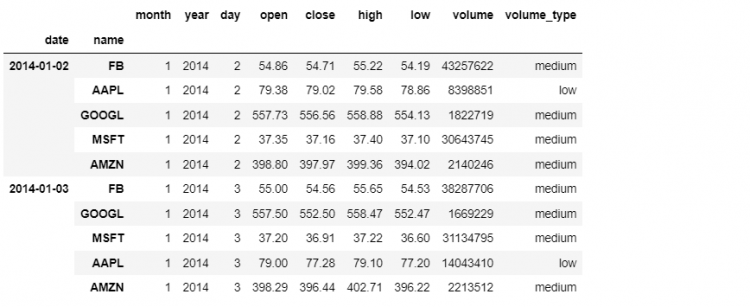
For example, let us say we want to find out the opening price for Google on January 1st, 2014. In other words, we will take the first day that we have in the DataFrame and retrieve the closing price of January 2nd, 2014.
Using the loc indexer
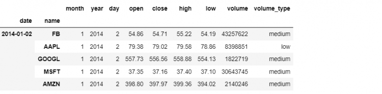
- STEP 1: Isolate the full dataset for that particular date, which is the outer label.
tech.loc['2014-01-02']- STEP 2: Extract the data for Google. This gives us a series containing all the values for Google at that date.
tech.loc['2014-01-02', 'GOOGL']

# Output
month                1
year              2014
day                  2
open            557.73
close           556.56
high            558.88
low             554.13
volume         1822719
volume_type     medium
Name: (2014-01-02, GOOGL), dtype: object- STEP 3: Append the
closeattribute in the given query to retrieve the closing price for the date. Hence, we get the closing price that was required.
tech.loc['2014-01-02', 'GOOGL'].close

# Output
556.56
Using the label in the loc indexer
Another method to accomplish the same result is to use the label that we have created. We can pass both the outer and inner labels of our DataFrame as a tuple to the loc indexer.
This will result in the seclusion of Google values at that particular date. Further, we will pass the close attribute for the desired output.
tech.loc[('2014-01-02', 'GOOGL'), 'close']

# Output
556.56
The iloc indexer does not consider the hierarchy of the data structure. This means that it won’t pay heave to whether the DataFrame has been created using multi-indexing or not. However, the loc indexer cares for the structure of the DataFrame.
Using the iloc indexer
If the same output needs to be generated using the iloc method, we can simply pass in the ordinal positions of the value to be retrieved as parameters.
tech.iloc[2,4]

# Output
556.56
Indexing Ranges and Slices
We looked at some ways to select values from a multi-index DataFrame, specifically by label or position, building on that knowledge, we will take a look at extracting sequences of slices of values.
Let us begin with the simple task of extracting multiple days from our tech stocks DataFrame. Using the loc indexer, if we need to select several dates, all we need to do is to pass in a list of labels containing those dates.
tech.loc[['2015-01-06', '2015-01-07']]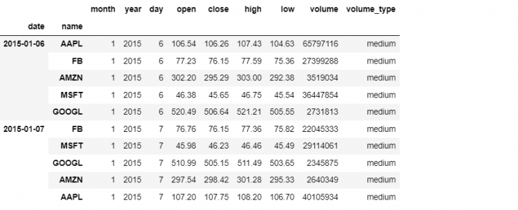
Pandas use the list of labels to extract from the outer level of our multi-index. If we simply want a subset of stock names we simply specify those in another list of index labels.
# Wrong Approach
tech.loc[['2015-01-06', '2015-01-07'], ['FB', 'AMZN']]
But we cannot pass on another list because Pandas throws an error “None of [Index([‘FB’, ‘AMZN’], dtype=’object’)] are in the [columns]” since the loc indexer perceives it as we are trying to index along the column dimension.
So instead, we need to wrap these two lists in a tuple containing two items, which is because our multi-index contains two levels.
tech.loc[(['2015-01-06', '2015-01-07'], ['FB', 'AMZN']), :]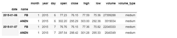
Slices in a Multi-Index DataFrame
In regular DataFrames or Series, we can slice our data structures by specifying a range of values separated by a column.
tech.loc['2017-01-03':'2017-01-31', 'open':'low']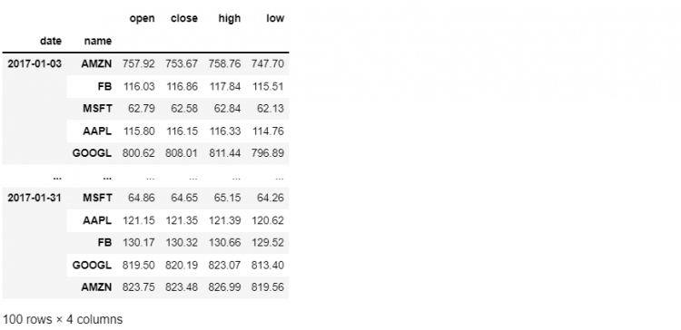
In this case, we are slicing across both dimensions of our dataset. We are selecting dates along with the outer level of our multi-index and we are also selecting a column slice from our column axis.
Now, if we want to get more specific and only isolate the Google data out of the five selections, we will be using the slice object.
To slice our DataFrame by a range of dates for only the Google stocks, we have to specify the date range in a stand-alone slice object, which is then wrapped in a tuple with our other index label, stock name.
tech.loc[(slice('2017-01-03', '2017-01-31'), 'GOOGL'), 'open':'low']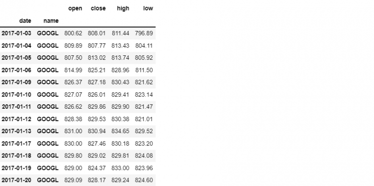
Now, let us assume, we need to find the open prices for FB and AMZN for all dates in our DataFrame.
tech.loc[(slice(None), ['FB', 'AMZN']), 'open']

# Output
date        name
2014-01-02  FB        54.86
2014-01-03  FB        55.00
                     ...
2019-08-21  AMZN    1819.39
2019-08-22  AMZN    1828.00
2019-08-23  AMZN    1793.03
Name: open, Length: 2842, dtype: float64
Cross Sections With xs
So far, we have seen various approaches for indexing hierarchical DataFrames. All of them are quite powerful and flexible but not the most intuitive in terms of syntax.
The xs method, in terms of functionality, is a subset of label-based indexing. The syntax of this method is quite straightforward.
For example, let us say we want to get the cross-section of our DataFrame for the first trading day in the year 2019. This can be accomplished using xs in the following manner.
tech.xs('2019-01-02')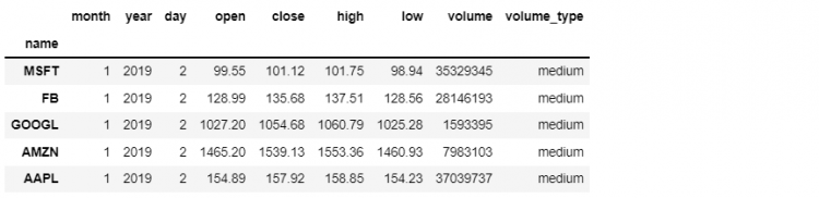
We have previously used the loc indexer to get the same result. However, now we want to select an element using the stock name instead. In this case, we will use the command mentioned below.
tech.xs('FB', level=1, drop_level=False)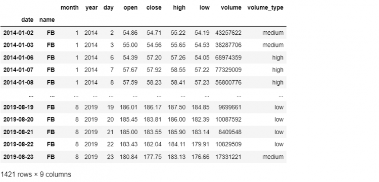
By default, the xs method excludes the level upon which selection is based. Thus we have set the drop_level parameter to False to get the selected level in the result.
Next, we can also select from multiple levels of our index at once by passing the same-sized tuples to both the key and level parameters. In the following example, we have used the first and the second level to select from our multi-index.
tech.xs(('2019-01-02', 'FB'), level=(0,1))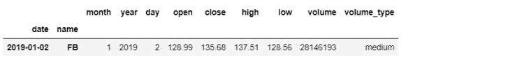
The Anatomy of a Multi-Index Object
We will be discussing exactly how a multi-index object is structurally put together in Pandas which will be very useful while working with or manipulating hierarchical DataFrames.
tech.index

# Output
MultiIndex([('2014-01-02',    'FB'),
            ('2014-01-02',  'AAPL'),
            ...
            ('2019-08-23', 'GOOGL'),
            ('2019-08-23',  'AMZN'),
            ('2019-08-23',    'FB')],
           names=['date', 'name'], length=7105)
A multi-index is like a data structure in itself, it has its specific attributes, sequence of values, and methods. The multi-index object can support very complex structures and hierarchies in a self-contained way.
We can even take an object from one DataFrame and pass it on to another. Now let us take and discuss one component at a time.
Names
The names attribute returns the two labels that we are indexing by. In our case, it is name and date.
tech.index.names

# Output
FrozenList(['date', 'name'])
Levels
nlevels is a list that contains all the range of values for labels in our multi-index.
tech.index.nlevels

# Output
2
This should be consistent with the length of the levels list of indices, which is:
len(tech.index.levels)

# Output
2
The highest level in our index is considered to be the left-most, for example, the highest level in our DataFrame is the date.
Therefore, the outer-level is level 0, and inwards towards the actual columns the levels keep increasing, which is why name is level 1.
tech.index.levels[0]

# Output
Index(['2014-01-02', '2014-01-03', '2014-01-06', '2014-01-07', '2014-01-08',
       '2014-01-09', '2014-01-10', '2014-01-13', '2014-01-14', '2014-01-15',
       ...
       '2019-08-12', '2019-08-13', '2019-08-14', '2019-08-15', '2019-08-16',
       '2019-08-19', '2019-08-20', '2019-08-21', '2019-08-22', '2019-08-23'],
      dtype='object', name='date', length=1421)
This displays all the dates in our DataFrame.
tech.index.levels[1]

# Output
Index(['AAPL', 'AMZN', 'FB', 'GOOGL', 'MSFT'], dtype='object', name='name')
Levshape
If we want to look at the length of each of our levels, we can use the levshape attribute, which stands for level-shape.
tech.index.levshape

# Output
(1421, 5)
Now this means we have 1421 dates by 5 names.
Values
Multi-indices are not just freely floating sequences of labels, they represent a tight coupling of hierarchies of labels. An easy way to look at the label combinations across our index levels is to access the values attribute on the multi-index itself.
tech.index.values

# Output
array([('2014-01-02', 'FB'), ('2014-01-02', 'AAPL'),
       ('2014-01-02', 'GOOGL'), ..., ('2019-08-23', 'GOOGL'),
       ('2019-08-23', 'AMZN'), ('2019-08-23', 'FB')], dtype=object)
Here, we get a list of tuples each containing two items, a date, and a stock name. If we had a three-level multi-index, we would get the third value in the tuple as well.
The values attribute is the sequence of all possible associations across each level of our multi-index.
Adding a Level in a Multi-Index
We have been working with two levels till now, date and name. Now we will be adding a new level in our DataFrame, let us say the volume_type. The volume_type is set to:
- high: If the volume is more than twice the average for that stock.
- low: If it is less than twice the average for that stock.
- medium: Otherwise.
There are a couple of ways to squeeze this categorical attribute within our multi-index.
Using the set_index method
Setting a new level using the set_index function is the most intuitive method.
tech.set_index('volume_type', append = True, inplace = True)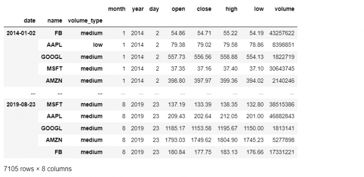
We are indicating in the command above, that we want the volume_type column to act as our index but not in a way that it replaces our existing index but rather, it appends it. The inplace parameter makes the changes stick to our original DataFrame.
The volume_type is now added to the third level of our multi-index.
tech.index.nlevels

# Output
3

# Isolating the 3rd Level
tech.index.levels[2]

# Output
Index(['high', 'low', 'medium'], dtype='object', name='volume_type')

tech.index.values

# Output
array([('2014-01-02', 'FB', 'medium'), ('2014-01-02', 'AAPL', 'low'),
       ('2014-01-02', 'GOOGL', 'medium'), ...,
       ('2019-08-23', 'GOOGL', 'medium'),
       ('2019-08-23', 'AMZN', 'medium'), ('2019-08-23', 'FB', 'medium')],
      dtype=object)
Since we introduced a new level, selecting by a label from the DataFrame will also look a bit different. Let us assume, we wish to select all the data from high volume trading days from January 2019.
We can still use the loc indexer but, now we need to specify a longer tuple.
tech.loc[(slice('2019-01-01', '2019-01-31'), slice(None), 'high'), :]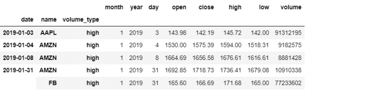
Taking another example, if we want to get all high-volume trading days. Using the cross-section method:
tech.xs(level=2, key = 'high')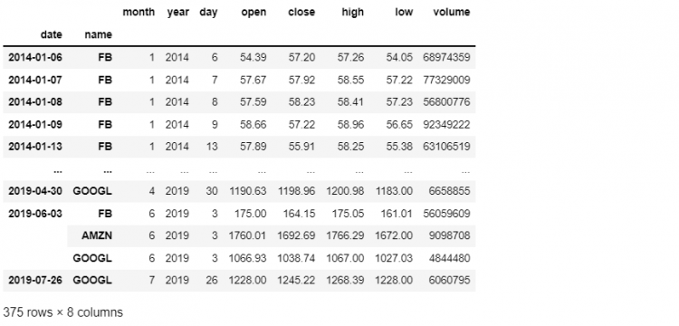
Shuffling the Levels
We saw how to add additional levels to our multi-index, but if we are not satisfied with the order in which these levels appear within our multi-index.
Taking an example, what if we wanted to make the newly added level volume_type come immediately after the first level i.e. date but before name.
One way to do this is to read the data again and set the index in a different order. There is also a better and quicker approach that operates on our existing multi-index, the swaplevel method.
tech.swaplevel(2,1)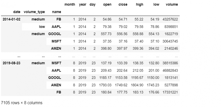
We call this method on a hierarchically indexed DataFrame and then we pass the two levels whose positions we want to be swapped or exchanged. This gives us a new multi-indexed DataFrame that has volume_type as the second level within the index.
The swaplevel method also works with label names instead of label positions. So, we can also say:
tech = tech.swaplevel('volume_type', 'name')
Unfortunately, this method does not have an inplace parameter, so if we want the changes to be applied to the underlying DataFrame we have to reassign our variable to point to new DataFrame returned by swaplevel.
In Pandas, there is a more powerful method that works with more than two levels at a time. What we have done so far is a simple positional swap of two levels, if we want to reorder more broadly the alternative is the reorder_levels method.
The reorder_levels method allows us to express a new order for the multi-index all in one go. We pass in a list of positions and we get a new DataFrame that follows that order.
tech.reorder_levels([2, 0, 1])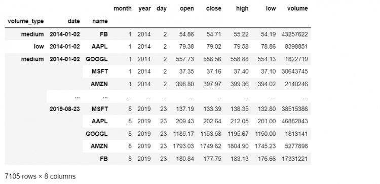
The reorder_levels method can be called on the hierarchically indexed DataFrame, as we did above, or on the multi-index directly. In that case, it returns a new multi-index with the labels ordered in the way they were specified.
tech.index.reorder_levels([2, 1, 0])

# Output
MultiIndex([('medium',    'FB', '2014-01-02'),
            (   'low',  'AAPL', '2014-01-02'),
            ('medium', 'GOOGL', '2014-01-02'),
            ...
            ('medium',  'AMZN', '2019-08-23'),
            ('medium',    'FB', '2019-08-23')],
           names=['volume_type', 'name', 'date'], length=7105)
Removing Multi-Index Levels
We have talked about adding new levels and even changing their order in our multi-index, now we will take a look at removing levels. Pandas recently introduced a method to perform the same, i.e. the droplevel method.
Let us say we want to exclude the volume_type level, i.e. position 1, we simply use:
tech.droplevel(1)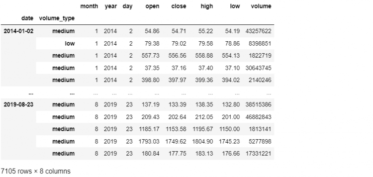
We get a new hierarchically indexed DataFrame from where the volume_type level has been removed. We notice one thing, the volume_type level is missing from both the levels columns and the general columns.
Unfortunately, there is no way to restore it as a regular column using the droplevel method. This is why we prefer using another method that is the reset_index.
The reset_index is a lot more powerful and flexible. Not only does it allow us to remove a given level, just like droplevel, but also restores it back to the DataFrame as a regular column.
tech.reset_index(level = 2)
This restoration is because reset_index has a drop parameter that controls this aspect of what we do with levels being removed. This drop parameter defaults to False, which is why we see it restored in the DataFrame. If we set this to true, the removed level is truly discarded just like the droplevel method.
Removing Multiple Levels
If we wish to remove several from our multi-index DataFrame at once, we could either remove those levels one at a time calling droplevel or reset_index functions separately, but fortunately both these levels accept lists of level names.
Let us say we need to remove both volume_type and name from the DataFrame, we can say:
- Using
drop_levelMethod
tech.droplevel(['volume_type', 'name'])

# Can also be used with positions
tech.droplevel([1, 2])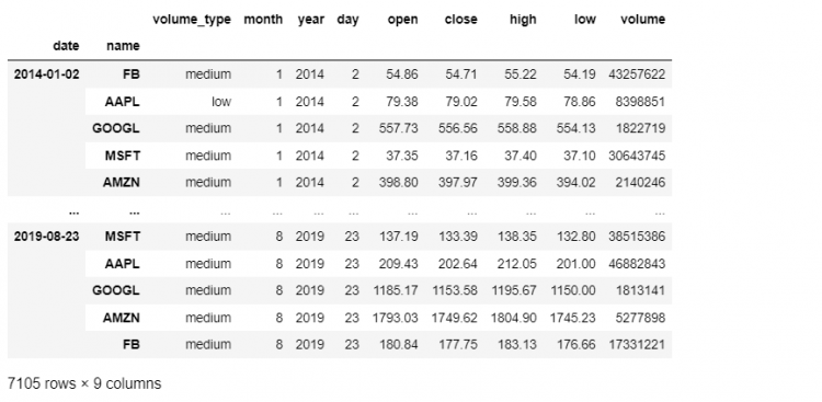
- Using
reset_indexMethod
tech.reset_index(level = ['volume_type', 'name'], drop = True)Totally Resetting the Index
For resetting the existing index and getting back a basic range index, we simply call the method reset_index method with no parameters on the DataFrame itself.
tech.reset_index()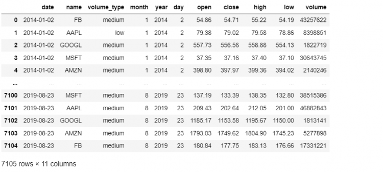
We get back the plain range index acting as our new index and all the previous levels that were a part of our multi-index got restored as regular columns in our DataFrame.
Sorting Multi-Indices
When we looked at slicing our multi-indexed DataFrame using labels, we combined multiple slice objects within a tuple. Let’s look at the following example:
tech.loc[(slice('2014-01-02', '2014-04-02'), slice(None), 'AAPL'), 'open':'low']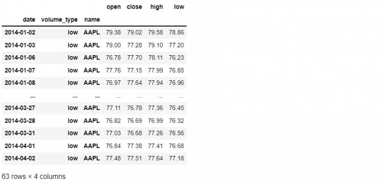
Here, we are selecting the open, close, high, and low prices for Apple for the first three months of trading in 2014 for all volume types. Now, what would happen if we wanted to select not just Apple but a slice going from Apple to Facebook.
If we use the following approach and wrap the names in a slice object, Pandas throws an “UnsortedIndexError: ‘MultiIndex slicing requires the index to be lexsorted“.
tech.loc[(slice('2014-01-02', '2014-04-02'), slice(None),
          slice('AAPL', 'FB')), 'open':'low']
The reason for this is that it is not very meaningful to talk about slicing a longer sequence of values that is not sorted or does not have an intrinsic order. Now we need to sort our index using the sort_index method.
tech.sort_index(inplace = True)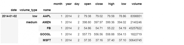
This command sorts all levels and saves the result in place. Now if we go to our previous command that was throwing an error, and re-execute it, everything works fine.
tech.loc[(slice('2014-01-02', '2014-04-02'), slice(None),
          slice('AAPL', 'FB')), 'open':'low']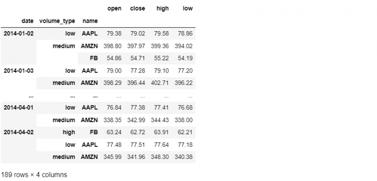
Advantages of using a sorted Multi-Index
- Improves retieval performance significantly.
- Enables slicing syntax.
- Overall a good practice while working with tabular data representations, including Pandas, Excel, SQL, etc.
The sort index method is the same that we’ve seen in practice, but for multi-index DataFrames specifically, we can fine-tune the sort using the level parameter.
For example, if we wanted the most recent dates to come on the top, i.e. we wish to sort only one level of our multi-index in descending order and the names in ascending order.
This can easily be done with the help of the sort_index method.
tech.sort_index(level = (0, 2), ascending = [True, False])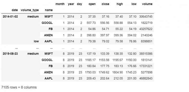
Multi-Index Methods
Apart from the methods we have discussed so far, it’s important to keep in mind that the multi-index object can also be manipulated as a stand-alone data structure. Henceforth, we will take a look at some methods that are only applicable to multi-index DataFrames.
To begin with, we will create a pointer called tidx. Then, we will call the index attribute of the DataFrame and assign its value to the newly created pointer. The index attribute gives us the multi-index.
tidx = tech.index

# Output
(MultiIndex([('2014-01-02',  'AAPL',    'low'),
             ('2014-01-02',  'AMZN', 'medium'),
             ...
             ('2019-08-23',    'FB', 'medium'),
             ('2019-08-23', 'GOOGL', 'medium'),
             ('2019-08-23',  'MSFT', 'medium')],
           names=['date', 'name', 'volume_type'], length=7105)
First of all, we will check whether this index is sorted. To do this we run the following command to confirm whether the index is sorted alphabetically:
tidx.is_lexsorted()

# Output
True
Now that we know that the index is sorted, we can proceed further. If we wish to modify the sort for a given level within our multi-index without touching the DataFrame itself, we can use the sortlevel method directly on the index.
tidx.sortlevel(0, ascending=False, sort_remaining=True)

# Output
(MultiIndex([('2019-08-23',  'MSFT', 'medium'),
             ('2019-08-23', 'GOOGL', 'medium'),
             ...
             ('2014-01-02',  'AMZN', 'medium'),
             ('2014-01-02',  'AAPL',    'low')],
            names=['date', 'name', 'volume_type'], length=7105),
 array([7100, 7102, 7104, ...,    0,    4,    1], dtype=int64))
As we can see from the mentioned example, the sortlevel method takes three parameters:
- The level that needs to be modified.
- Whether it should be sorted in ascending order or not.
- Whether the remaining levels should be sorted or not.
Unlike the sortindex method which is applied to the complete DataFrame, the sortlevel method is applied to the multi-index. We can also sort multiple levels at once.
Consider the following example.
tidx.sortlevel((0, 1, 2), ascending=[True, True, False])

# Output
(MultiIndex([('2014-01-02',  'AAPL',    'low'),
             ('2014-01-02',  'AMZN', 'medium'),
             ...
             ('2019-08-23', 'GOOGL', 'medium'),
             ('2019-08-23',  'MSFT', 'medium')],
            names=['date', 'name', 'volume_type'], length=7105),
 array([   1,    4,    0, ..., 7104, 7102, 7100], dtype=int64))
Now, let us take a look at how to modify the aesthetics of the multi-index.
tech.head()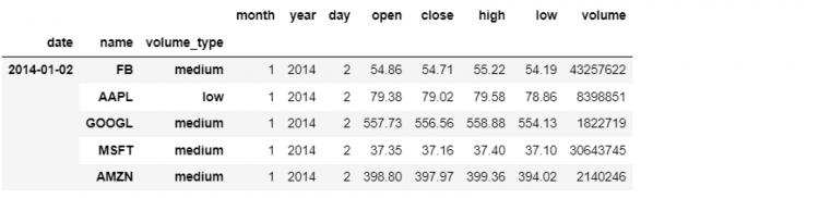
In the following example, we will use the set_names method on the multi-index directly. This method takes a list of labels that are equal in length to the number of labels in our multi-index.
tidx.set_names(['Trading  Date', 'Volume Category', 'Ticker'])

# Output
MultiIndex([('2014-01-02',    'FB', 'medium'),
            ('2014-01-02',  'AAPL',    'low'),
            ...
            ('2019-08-23',  'AMZN', 'medium'),
            ('2019-08-23',    'FB', 'medium')],
           names=['Trading  Date', 'Volume Category', 'Ticker'], length=7105)
Reshaping with stack Method
We will take a look at the stack method which is widely used alongside pivot tables, but for now, let us talk about it in a multi-index concept.
The stack method is used to take the column axis and pivot or rotate it into the inner-most level of the index.
So starting with our tech dataset, if we call stack on our multi-index DataFrame we end up with a series where the index now includes our column labels as a new level within our multi-index. Let us assign this to a new variable stacked for ease of access.
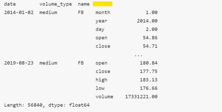
stacked = tech.stack()

# Output
date        volume_type  name
2014-01-02  medium       FB    month            1.00
                               year          2014.00
                               day              2.00
                               open            54.86
                               close           54.71
                                            ...
2019-08-23  medium       FB    open           180.84
                               close          177.75
                               high           183.13
                               low            176.66
                               volume    17331221.00
Length: 56840, dtype: float64
We went from DataFrame to Series which may seem like we lost a dimension but instead, it is a transfer of dimension from the column axis to a wider multi-index. We went from a three-level multi-indexed DataFrame with a one-level column axis to a four-level multi-index series containing a single sequence of values.
type(stacked)

# Output
pandas.core.series.Series

stacked.index.nlevels

# Output
4
Renaming the Levels
We notice the stacked variable has a gap which indicates that the level does not have a name, so let us quickly fix that using the set_names methods.
- STEP 1: Let us first isolate the names.
stacked.index.names

# Output
FrozenList(['date', 'volume_type', 'name', None])
FrozenList is a data structure in Pandas that is immutable. Therefore, it is impossible for us to just change its content. The only way to change it is by creating a new instance object.
We see that the last attribute is None which is responsible for no name in our series. To fix this we will use set_names.
- STEP 2: Let us assign the FrozenList to a variable
names.
names = stacked.index.names- STEP 3: We will now set the names of the levels using the
set_namesfunction by modifying thenamesvariable.
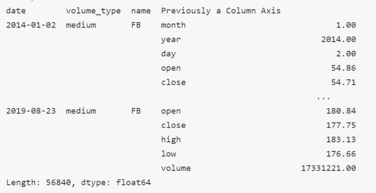
stacked.index.set_names([*names[:-1], 'Previously a Column Axis'], inplace = True)

# Output
date        volume_type  name  Previously a Column Axis
2014-01-02  medium       FB    month                              1.00
                               year                            2014.00
                               day                                2.00
                               open                              54.86
                               close                             54.71
                                                              ...
2019-08-23  medium       FB    open                             180.84
                               close                            177.75
                               high                             183.13
                               low                              176.66
                               volume                      17331221.00
Length: 56840, dtype: float64
Reshaping with unstack Method
In the previous section, we have learned the use of the stack method which takes a column axis and chops it into our index labels. The unstack method does the exact opposite of that.
The unstack method takes the innermost level of a multi-index and moves it back to the column axis. Let us use the unstack method on our stacked dataset.
As we can see, the innermost level of the dataset used to be a column axis. We will use the unstack method to take this innermost level back to the column dimension. We can simply use the following command to achieve this.
stacked.unstack()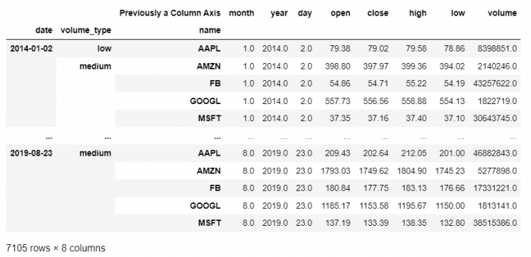
Hence, we have retrieved our previous DataFrame from the modified dataset. Furthermore, the function can be called multiple times.
stacked.unstack().unstack()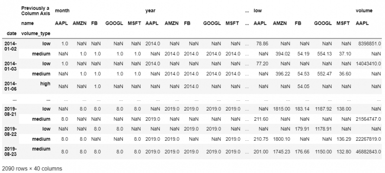
By running the above piece of code, we end up creating a multi-index column axis. We now have two levels within our column dimension. Thus, this DataFrame now has two-level multi-indices on both the index and the column dimension.
However, we have created gaps in our DataFrame which are represented by NaN due to the lack of adequate information. However, the fill_value parameter of the unstack method allows us to replace these gaps with the desired value.
Moreover, we can also specify exactly what level we want to operate on while using the mentioned methods. Let us consider an example where we will unstack the Volume Category level, instead of the innermost level.
stacked.unstack(level=1)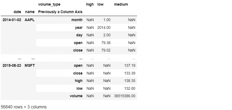
Another way to do this is by mentioning the name of the level to be unstacked.
stacked.unstack(level = 'name')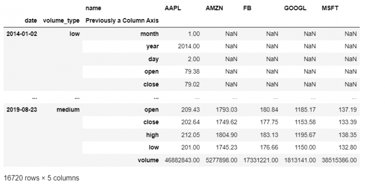
Hence, we receive the DataFrame having the input level moved to the column dimension.
Multi-Level Columns using transpose
For manually creating a multi-level column axis we need to combine the set_index with transpose method. We know:
set_indexenables us to create a hierarchical index.transposeswaps the DataFrame such that the columns becomes its rows and vice versa.
Let us say, we are interested in reshaping our tech DataFrame. Let us set the date and volume_type as our indices.
tech.set_index(['date', 'volume_type'])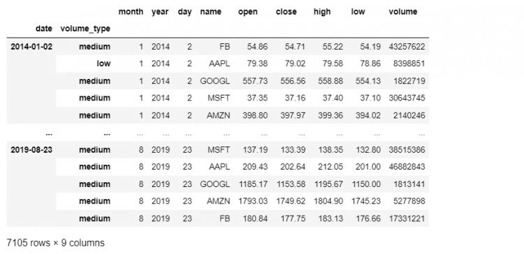
Now we have our multi-index, at this point, we use transpose in order to flip this DataFrame over, to make our index become our column. We will end up with two multi-index columns.
Hence, we get a hierarchical index using set_index and transpose functions.