Advanced DataFrames

We will take a closer look at the advanced indexing using binary operators and multiple boolean conditions, exploring some computer science concepts which include bitwise operators and how modern computers represent numbers.

Sorting, indexing, and looking up values to reorder our records into customized logic. We will be discussing pruning operations related to duplicate and null values, and how to reshape our DataFrame.

Indexing with Boolean Masks

We have already discussed indexing with boolean masks for DataFrames before. The key concept while using a boolean mask is a 2 step process:

• STEP 1: To generate a sequence of booleans.
• STEP 2: Using this boolean sequence in [] or .loc[]

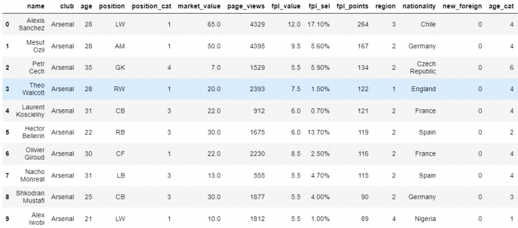
Considering a large sample DataFrame of famous soccer players:

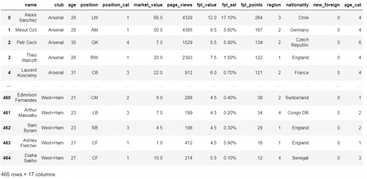
Now let us consider, we need to find out the players who have a market value greater than 60 million.

• STEP 1: Generating the sequence of booleans.

# Using the comparison operator we obtain a boolean series
df.market_value > 60

# Output
0       True
1      False
2      False
       ...  
463    False
464    False
Name: market_value, Length: 465, dtype: bool

We have now obtained a series of booleans. To complete this selection, we simply need to pass this boolean series into the DataFrame.

• STEP 2: Using this boolean sequence in [] or .loc[]

# Passing the boolean series into the DataFrame
df[df.market_value > 60]

# To find out the total number of players fitting into the category
df[df.market_value > 60].shape

# Output
(5, 17)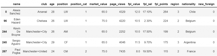

More approaches to Boolean Masking

Using the isin Function

Now let us take another example, suppose we need to find all the defenders in our DataFrame. (We have our defender codes as LB, CB, and RB.)

# Checking whether the position is in the array of defender codes.
df.position.isin(['LB', 'CB', 'RB'])

# Output
0      False
1      False
2      False
       ...  
463    False
464    False
Name: position, Length: 465, dtype: bool

Now, we need to pass on this boolean sequence into our DataFrame.

# Passing the boolean series into the DataFrame
df[df.position.isin(['LB', 'CB', 'RB'])]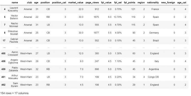

Using the between Function

Taking another example, let us consider we need to find out the players having a market value between 40 and 50 million. We will do this using the between() function.

# Using the comparison operator we obtain a boolean series.
df.market_value.between(40,50)

# Output
0      False
1       True
2      False
       ...  
463    False
464    False
Name: market_value, Length: 465, dtype: bool

Now we will pass this to the DataFrame to print all the players having a market value between 40 and 50.

# Passing the boolean series into the DataFrame
df[df.market_value.between(40,50, inclusive=False)]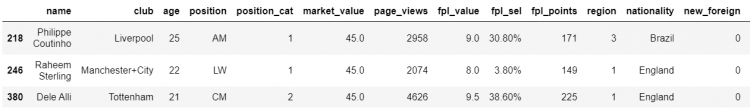

Using the comparison functions

The Pandas library has functions for every comparison operator we use. The comparison operators and their corresponding Pandas methods are given in the following table.

Comparison Operators	Pandas Method
<	.lt()
<=	.le()
>	.gt()
>=	.ge()
==	.eq()

Taking an example, let us assume we need to find all the players having an age less than equal to 25.

# Checking whether the position is in the array of defender codes.
df.age.le(25)

# Output
0      False
1      False
2      False
       ...  
463     True
464    False
Name: age, Length: 465, dtype: bool

Passing the obtained boolean sequence into the DataFrame.

# Passing the boolean series into the DataFrame
df[df.age.le(25)]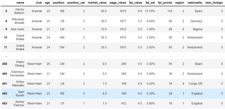

Binary Operators with Booleans

Binary operators are just like the other operators like +, -, *, / etc. The only difference is that the binary operators work on the binary representation of the value, on the individual bits.

Two of the major operators are:

• Binary OR – |
• Binary AND – &

Binary OR operator

The truth table for the Binary OR operator is given as follows:

A	B	A|B
0	0	0
0	1	1
1	0	1
1	1	1

Binary AND operator

The truth table for the Binary AND operator is given as follows:

A	B	A|B
0	0	0
0	1	0
1	0	0
1	1	1

Let us create a Pandas boolean series, having alternative True and False.

# Creating a boolean series
t = pd.Series([True if i%2 ==0 else False for i in range(10)])
t

# Output
0     True
1    False
2     True
3    False
4     True
5    False
6     True
7    False
8     True
9    False
dtype: bool 

To try out the boolean operators on the series, we create another boolean series having all False.

# Creating another boolean series
f = pd.Series([False for i in range(10)])
f

# Output
0    False
1    False
2    False
3    False
4    False
5    False
6    False
7    False
8    False
9    False
dtype: bool

Using the Binary OR operator on the two series:

# t OR f
t | f

# Output
0     True
1    False
2     True
3    False
4     True
5    False
6     True
7    False
8     True
9    False
dtype: bool

Using the Binary AND operator:

# t AND f
t & f

# Output
0    False
1    False
2    False
3    False
4    False
5    False
6    False
7    False
8    False
9    False
dtype: bool

There are several other binary operations, two of them we are going to discuss are given below:

• XOR – The Exclusive OR
• Complement

Binary XOR operator

The XOR operator, which stands for Exclusive OR. It gives True only when the inputs are different and False when the inputs are similar. The XOR operator in python is represented as ^ (caret symbol).

The truth table for the Binary XOR operator is given as follows:

A	B	A^B
0	0	0
0	1	1
1	0	1
1	1	0

# t XOR f
t ^ f

# Output
0     True
1    False
2     True
3    False
4     True
5    False
6     True
7    False
8     True
9    False
dtype: bool

The Two’s Complement

The Two’s Complement is represented as ~ (tilde symbol) in python. This operator is very useful in Boolean Series, for finding the opposite of the series. All of these operators act on the Bits of a number.

Let us take an example to understand it further:

# Taking two's complement
~ True

# Output
-2

~ False

# Output
-1

This provides some surprising results because it is related to how computers represent numbers. It gives the binary complement the number. It inverts the bits representing the number, as shown in the figure below:

Combining conditions using operators

While performing multi-condition selections, we combine several boolean series using the binary operators, discussed above. Let us understand this using an example.

Suppose we need to find all the left-backs who are 25 or younger. We will do this using two conditions and combine them using the AND binary operator.

# Combining conditions using AND operator
df[(df.position == 'LB') & (df.age <= 25)]

NOTE: Always remember to wrap the two conditions, connected by the binary operator, in separate parenthesis.

Let us take another example, let us say we want to retrieve the players who are left-backs, 25 years or younger, having a market value above 10 million, and who are not from Arsenal or Tottenham clubs. Now we have four conditions to look for:

# Combining four conditions using AND operator
df[
    (df.position == 'LB') &
    (df.age <= 25) &
    (df.market_value >= 10) &
    ~(df.club.isin(('Tottenham', 'Arsenal')))
]

Conditions as Variables

The multi-line expression we came across in the above example is quite difficult to read. To avoid such cases we can always refactor our conditions into stand-alone variables. Especially when we need to compose an indexing logic that involves several conditions, it is always a good idea to refactor.

Let us take another example to understand using conditions as variables. Let’s consider we need to find all the Arsenal right-backs and Chelsea goalkeepers.

• STEP 1: Let us create a variable as arsenal_player which stores the boolean series for all the players belonging to the Arsenal club.

# Creating the 'arsenal_player' variable
arsenal_player = df.club == 'Arsenal'

arsenal_player

# Output
0       True
1       True
2       True
       ...  
463    False
464    False
Name: club, Length: 465, dtype: bool

• STEP 2: We will be creating another variable to store the boolean list of all the players who are on the position “RB” as right_back.

# Creating the 'right_back' variable
right_back = df.position == 'RB'

right_back

# Output
0      False
1      False
2      False
       ...  
463    False
464    False
Name: position, Length: 465, dtype: bool

• STEP 3: For the Chelsea Goalkeepers part, we are going to combine both the conditions to one variable. Therefore, we make another variable as chelsea_and_GK which is for the players who are Goalkeepers from the Chelsea club.

# Creating the 'right_back' variable
right_back = df.position == 'RB'

right_back

# Output
0      False
1      False
2      False
       ...  
463    False
464    False
Name: position, Length: 465, dtype: bool

• STEP 4: Now all we need to do is to index the DataFrame by passing the above conditions in square brackets or the loc indexer.

# Indexing the DataFrame using the conditions as variables
df.loc[arsenal_player & right_back | chelsea_and_GK]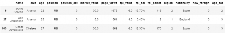

2D Indexing

In the last section, we have discussed Boolean Indexing in the context of extracting rows. Our indexing has only operated on the index axis, the axis zero, which is the default behavior in Pandas.

When working with DataFrames, we are working with two dimensions, and therefore we certainly have an option of indexing along the other axis as well.

The loc parameter method

Let us take an example, consider we need to find the players from the Chelsea club who are 23 years or younger.

• STEP 1: Let us begin my forming the conditions and storing them in a seperate variable chelsea_23under

# Creating the 'chelsea_23under' variable
chelsea_23under = (df.club == 'Chelsea') & (df.age.le(23))

chelsea_23under

# Output
0      False
1      False
2      False
       ...  
463    False
464    False
Name: position, Length: 465, dtype: bool

• STEP 2: To do the selection, we simply pass the above variable to the square brackets in the loc condition.

# Printing all the chelsea_23under players.
df[chelsea_23under]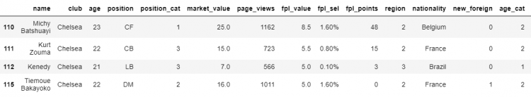

• STEP 3: In order to index the retrieved data according to the required columns, we specify the columns in a list as a parameter to the loc attribute.

# Creating the 'chelsea_23under' variable with column parameters.
df.loc[chelsea_23under, ['position', 'market_value']]

This is the most intuitive way to go about the selection from the column axis, but it is not very flexible. We have another method to index the DataFrame according to the column axis.

The startswith method

Taking another example where we need to find out all the column names that begin with ‘p‘.

• STEP 1: We use the DataFrame.columns attribute and use the startswith function, that will go through all the column labels and check whether they start with ‘p’ and returns a boolean list. Assign this list to a variable ‘p_cols‘.

# Creating the 'p_cols' variable
p_cols = df.columns.str.startswith('p')

p_cols

# Output
array([False, False, False,  True,  True, False,  True, False, False,
       False, False, False, False, False, False, False, False])

• STEP 2: Now all we need to do is to pass this variable to the loc indexer as a parameter.

# Creating the 'chelsea_23under' variable with column parameters.
df.loc[chelsea_23under, p_cols]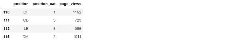

The chaining method

The third method to index according to the columns is the chaining method, where we chain two square brackets.

# Chaining two square brackets for indexing.
df[chelsea_23under]['position']

# Output
110    CF
111    CB
112    LB
115    DM
Name: position, dtype: object

Here, the first square bracket selects the DataFrame slice, containing all the columns and the second square bracket selects a single column from that.

This may appear to be equivalent to the loc method but in reality, the bracket method chaining method will always be slower, since the method get_item gets called twice. Therefore it is recommended to avoid using the chaining method as it may affect the runtime of the program.

Fancy Indexing with Lookup

The fancy indexing involved passing multiple labels all at once. The fancy indexing is similar to the basic label-based indexing, but instead of using single labels, we specify a list or a tuple of labels.

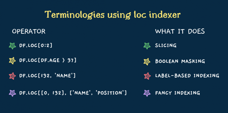
We will be talking about a Pandas method which is dedicated to fancy indexing and item selection and is more effective and quicker. This method is called lookup.

The lookup method takes a specific or a list of lookup labels and column labels and then it returns the value or values associated with each pair of labels.

Let us take an example where we need to find the value corresponding to the index label 450 and the column label ‘age‘.

# Fancy indexing using the lookup method
df.lookup([450], ['age'])

# Output
array([30], dtype=int64)

Loc vs the Lookup Method

We will consider a basic label-based selection using the loc indexer with some fancy indexing since we will be passing a list of index labels as well as a tuple of column labels.

# Fancy indexing using the loc method
df.loc[[0, 132], ('name', 'market_value')]

It gives us back a 2×2 DataFrame slice. Now let us compare this with what we get from the lookup method.

# Fancy indexing using the lookup method
df.lookup([0, 132], ['name', 'market_value'])

# Output
array(['Alexis Sanchez', 6.0], dtype=object)

Using the lookup method, we do not get back a DataFrame. Instead, we have an array of two items containing only the values that correspond to the row and column labels that we specified above.

Thinking of the parameters as label coordinates, the specifier row, and specifier column, and for that pair of labels, we get back a specific value.

So in the above lookup function, we have done this twice:

• Once with the 0 index label and the column ‘name’. Which gives us ‘Alexis Sanchez’, the first item in the array.
• The second time with the index label as 132 and the column ‘market_value’ and since they intersect at the value 6.0 which becomes our second item.

In reality, the lookup method is most useful when we already have a collection of labels that we want to select to do the DataFrame selection.

Sorting by Index and Column

Sorting by a particular value is not the only way to sort the DataFrame. We occasionally also find the need to sort the DataFrame by index, usually for the indices we create.

Let us set the index of our existing DataFrame using the set_index method.

# Setting Index of the DataFrame
df.set_index('name', inplace = True)

# Printing the DataFrame
df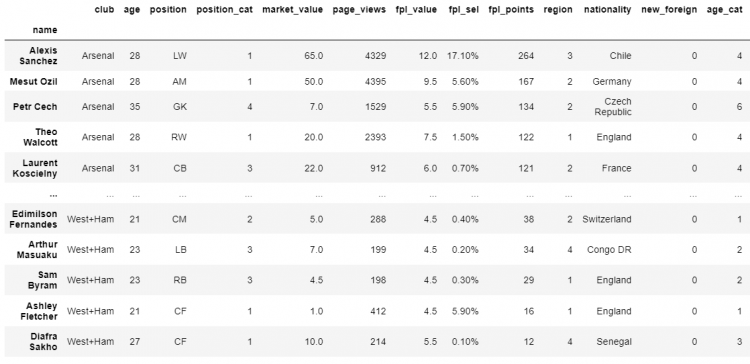

Now to order the Index according to the alphabetical order. In Pandas, it is very quick and easy to fix the unordered index using the sort_index method.

# Sorting the index of the DataFrame
df.sort_index(inplace = True)

# Printing the DataFrame
df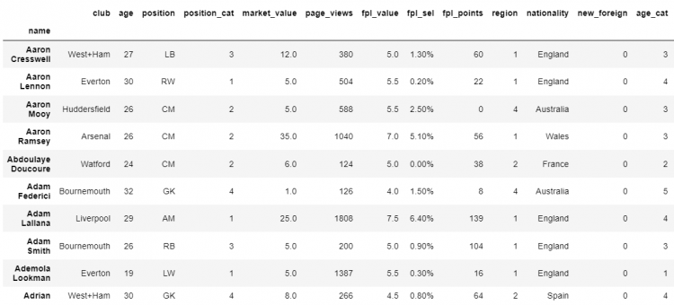

If we want the changes to be permanent in the DataFrame, we can set the inplace parameter to be True.

The sort_index method also helps us to sort our columns. Now, in addition to ordering our index axis, we also want to sort our column axis. We can do this using the sort_index method, all we have to do is to change the axis parameter, from the default of 0 to 1.

# Sorting the index of the DataFrame
df.sort_index(axis=1)

# Printing the DataFrame
df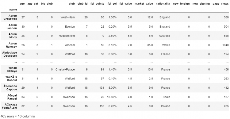

Sorting vs Reordering a DataFrame

We have sorted the DataFrame by values, index, and columns. Both the sort_values and sort_index methods contain several parameters that enable us to customize the specifics of how we want to carry out the sorting.

We have two fundamental ways of sorting:

• Ascending or in alphabetical order
• Descending order or in non-alphabetical order

Now, if we want to reorder more precisely in a DataFrame, according to a specified order, we can use the reindex method.

Let us begin by isolating a chunk of our DataFrame, using the iloc indexer and store it in a variable as df_lite.

# Slicing the DataFrame
df_lite = df.iloc[:4, :4]

# Printing the Sliced DataFrame
df_lite

Let us define a format we want our data to be reflected in, let’s say:

• row order: 2, 1, 3, 0
• column order: age, name, position, club

We cannot do this using the sorting method, so have to use the reindexing method.

# Reindexing using the format defined
df_lite.reindex(index = [2, 1, 3, 0], columns = ['age', 'name', 'position', 'club'])

Even if we use the same command on the entire DataFrame, we will get the same result without any errors.

# Reindexing the entire DataFrame using the format defined
df.reindex(index = [2, 1, 3, 0], columns = ['age', 'name', 'position', 'club'])

Now, let us suppose we need to get all the columns and have them alphabetically ordered.

# Reindexing to get all columns alphabetically ordered.
df.reindex(index = [2, 1, 3, 0]).sort_index(axis=1)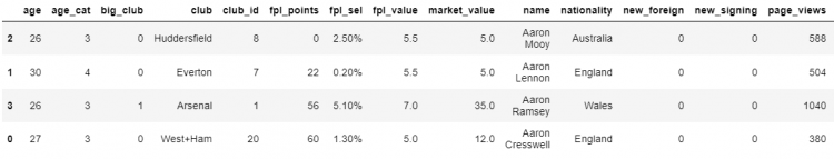

Identifying Duplicates in a DataFrame

In real-world scenarios, we often have to work with imperfect DataFrames, having duplicate values. This is why tools like Pandas are so popular among data analysts and scientists for handling, manipulating, and organizing such data.

Our example DataFrame does contain some duplicate records too. Duplicate values would be when the records have the same values across all columns.

This might cause a lot of problems, let’s say we need to find an average or aggregate calculation. If we have the same redundant value showing up multiple times, the resulting calculation will come out incorrectly.

An easy way to identify duplicate records in Pandas is by using the duplicated method.

# Identifying duplicate records using the duplicated function.
df.duplicated()

# Output
0      False
1      False
2      False
       ...  
463    False
464    False
Length: 465, dtype: bool

This method returns a boolean series. Now using the boolean masking method, we will pass this boolean series to select the duplicated items from the DataFrame.

# Selecting all the duplicated elements from the DataFrame
df[df.duplicated()]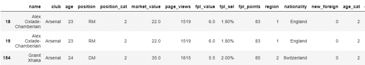

Specifying subsets to check duplicates

Sometimes we might fall into situations where we have duplicate values but a different value in a particular column that is making it look unique. In such cases, we need to have the ability to define precisely what constitutes a unique value.

In Pandas, we have an option to specify the subset of columns that should be considered to check the redundancy of the elements in a DataFrame. This can be achieved using the subset parameter.

Let us define that we need to characterize the unique elements by their club, age, position, and the market_value.

# Selecting all the duplicated elements using a subset
df.duplicated(subset = ['club', 'age', 'position', 'market_value'])

# Output
0      False
1      False
2      False
       ...  
463    False
464    False
Length: 465, dtype: bool


# Printing the duplicate elements
df.loc[df.duplicated(subset = ['club', 'age', 'position', 'market_value'])]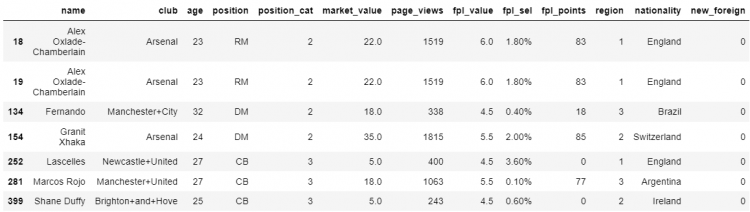

Labeling elements as duplicates

Now comes the question, how to find out which occurrence is original and which ones are the duplicate. Most often, also the default for Pandas, we treat the first occurrence of the element as original and every following similar index as the duplicate.

But this is not the only option available for us. If we order by a different parameter, the order of the appearance of the duplicates might change, which implies that this assumption has no intrinsic logic of its own.

To change this, we can use the keep parameter.

# Keeping the first occurrence of the duplicates
df.loc[df.duplicated(subset = ['club', 'age', 'position', 'market_value'], keep='first')]

The keep parameter takes in first, last, or False. The keep parameter by default is first, which means that Pandas considers the first value as the original and any duplicate value following it is duplicate.

Another option we have is last, which is exactly the opposite of the first. It means that in a set of repeating values, the last will be considered as the original value, and everything preceding it will be marked as a duplicate.

NOTE: The duplicated method parameters first and last does not change the shape of the DataFrame. We are only affecting the labeling of the DataFrame using this method.

There is also a third option which is boolean False. Setting the keep parameter to false indicates Pandas that all repeating values need to be treated as duplicates. Labeling keep to false does change the shape of the DataFrame since it treats all values to be duplicated.

Removing Duplicates in a DataFrame

We can remove duplicate values in a table using the drop_duplicates method, which returns the copy of the DataFrame where the duplicate values have been removed.

This method also has a keep parameter that takes in first, last, or False.

# Dropping duplicates keeping the first occurrence
df.drop_duplicates(keep = 'first')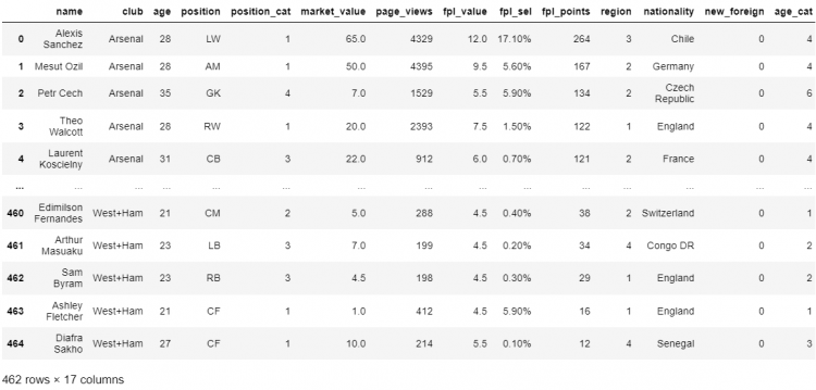

Now after removing the duplicates if we want to extract a particular column and perform aggregate calculations, we use the following approach.

For example, we need to find the aggregate market value of all the soccer players in the table after removing the duplicates.

# Dropping duplicates and finding the mean of market_value
df.drop_duplicates(keep = 'first').market_value.mean()

# Output
11.026252723311545

Let us compare the original mean and the mean after dropping the duplicates.

# Finding the original mean of market_value
df.market_value.mean()

# Output
11.125649350649349

This means that both of the means differ by almost 0.1 which is 1%, which is not a huge change in this case but it could be a lot worse in the case of DataFrames having a large number of duplicates or duplicates having extreme values.

Removing DataFrame Rows

Another approach for removing duplicates can be with the help of removing DataFrame rows. Firstly, we would have to identify the records that we want to remove and exclude all or some of them separately.

In our example DataFrame, we have 3 duplicate values. Let us assume, we want to remove one of these values and keep the other two. In that case, the drop_duplicates method won’t work here.

We can simply rely on the drop method to remove the specified number of rows from our DataFrame.

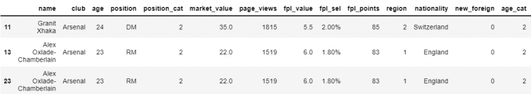
# Dropping the row having index 13
df.drop(labels = 13, axis = 0)

# Can also be written as df.drop(index = 13)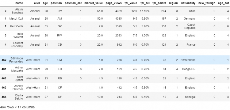

The drop method returns a copy of the DataFrame where the specified row is removed. If we have multiple rows to be removed, we can simply pass a list of the indices of all the rows as a parameter.

Removing DataFrame Columns

Using the drop method

We can use the drop method to remove columns of the DataFrame as well. All we need to do is to change the axis parameter of the drop method to 1 or ‘columns‘.

Let us take an example to remove the columns ‘age‘ and ‘market_value‘ from our sample DataFrame.

# Dropping the columns having index 'age' and 'market_value'
df.drop(labels=['age', 'market_value'], axis=1)

# Can also be written as df.drop(columns=['age', 'market_value'])

Using the pop method

The pop function takes in the column label we need to remove from the DataFrame. There are 3 points of difference to note about using this method:

• The pop method does not return the DataFrame with the column removed as in the drop method. Instead, it returns the removed column values in the form of a series.
• The pop function works at a single column at once.
• The pop function modifies the underlying DataFrame. Which means the function operates inplace.

Let us assume we need to permanently remove the ‘club‘ column from the DataFrame. We can use the following pop command to perform this function.

# Permanently dropping the 'club' column
df.pop('club')

# Output
0       Arsenal
1       Arsenal
2       Arsenal
         ...   
463    West+Ham
464    West+Ham
Name: club, Length: 465, dtype: object

Using reindexing

Another method of removing columns and rows is reindexing the DataFrame by leaving out several unwanted rows or columns. The reindex method crafts a new DataFrame which only reflects the labels we specify.

Let us consider we need to slice a DataFrame that does not include labels page_views, region, and position.

• STEP 1: We define a new variable ‘unwanted_values‘ and assign a list of all the column or row values we want to exclude from the new DataFrame, which in this case are page_view, region, and position.

# Defining the unwanted variables.
unwanted_values = ['page_views', 'region', 'position']

• STEP 2: Reindexing using the DataFrame with the difference of the original set of indices and the specified set, i.e. the unwanted_values.

# Reindexing using the Difference
df.reindex(columns = set(df.columns).difference(unwanted_values))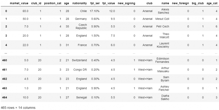

Null Values in a DataFrame

Null Values or the Null Markers, more commonly known as NaN refer to the gaps in the data of a DataFrame. The isna method is used to return a boolean series with True for all the elements containing a null value.

When using the isna method on a DataFrame, we get back a new DataFrame where each value is removed and replaced by a boolean indicating whether the value is NaN or not.

Calculating the total null values in a DataFrame

To quickly count the number of NaN in the DataFrame, we can use a very performant NumPy function count_nonzero.

# Function to count all the NaNs in a DataFrame.
np.count_nonzero(df.isna())

Finding out all the null records

To find out all the elements containing null values, first, we need to extract the values from the boolean DataFrame to create a boolean array of arrays.

• STEP 1: To get an array of arrays we use the following isna command.

# Finding an array of boolean arrays
df.isna().values

# Output
array([[False, False, False, ..., False, False, False],
       [False, False, False, ..., False, False, False],
       ...,
       [False, False, False, ..., False, False, False],
       [False, False, False, ..., False, False, False]])

• STEP 2: Now we can pass on the above array of boolean arrays to the DataFrame to retrieve all the elements having null values.

# Finding the elements having null values
df[df.isna().values]

Handling DataFrame Null Values

Filling or replacing the null values

Null values usually indicate a gap in the data, this could be the information that was lost, not available, or incorrectly recorded. So, we can fill or replace these null values with something more meaningful and the fillna method is really useful to accomplish that.

The fillna method takes in the new value we need to replace the null values with, and returns a copy of the DataFrame.

# Replacing all the null values in the DataFrame
df.fillna('something meaningful').loc[[30, 192, 195]]

In reality, our needs might be a bit more sensitive to the context. For example, if we want any null in the market_value should at least be replaced with a numerical value. To be able to do this, we could use a dictionary syntax of the fillna method.

Therefore, instead of passing a string, we pass on a dictionary that has different values associated with different keys.

# Replacing all the null values in market_value and position.
df.fillna({
    'market_value': 100,
    'position': 'RM'
}).loc[[30, 192, 195]]

Excluding or dropping the null values

An entirely different approach to deal with null values is to simply exclude them. For this, we have the dropna method. The dropna method on a DataFrame returns a new DataFrame which excludes rows containing the null values. This means the entire DataFrame rows are removed if any of the values contain a single null.

# Dropping all the null values in market_value and position.
df.dropna(axis = 1, how = 'any').loc[[30, 192, 195]]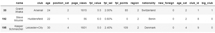

Calculating Aggregates in a DataFrame

The aggregate functions become useful when we wish to group our values along with several attributes. The agg method is the short form for the aggregate and it accumulates and aggregates the output of the function that we specify and collects the entire axis in a single value.

The agg function can be used to find the following:

• Mean
• Median
• Product
• Sum
• Min
• Max
• Standard Deviation
• Variance
• Mean Absolute Deviation

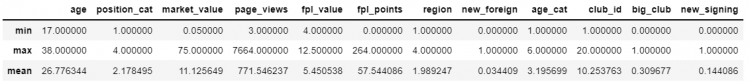
Let us find out the aggregate mean function on the entire DataFrame.

# Finding the mean of all columns using the agg function.
df.agg('mean')

# Output
age              26.776344
position_cat      2.178495
market_value     11.125649
...
club_id          10.253763
big_club          0.309677
new_signing       0.144086
dtype: float64

We can also pass in a list of agg functions, which would further give us a DataFrame where the values corresponding to every agg function across all numeric columns are reflected.

For example, we want to find an aggregate of min, max, and mean for all the numeric columns, we use the following approach to retrieve a DataFrame.

df.select_dtypes(np.number).agg(['min', 'max', 'mean'])

The select_dtypes function helps us to select distinct data types from the DataFrame.

Same Shape Transforms

Pandas also has a dedicated method used for applying constant functions to the entire DataFrame. The transform method also guarantees that the original shape of the DataFrame doesn’t change during the transformations.

Let’s say we want to convert our market_value and fpl_value from one currency to another, from USD to Euros.

• STEP 1: We need to have a conversion rate or an fx rate and isolate the slice of the DataFrame we want to perform the transformation on.

# usdeur conversion rate = 0.85

# We need to perform the transformation on the following slice
df.loc[: , ['market_value', 'fpl_value']]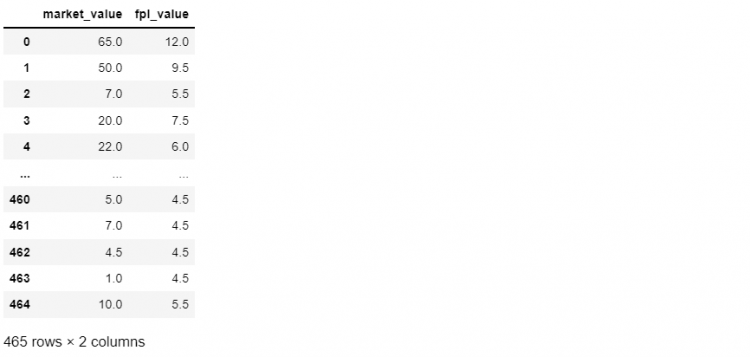

• STEP 2: Applying the transform function with an inline lambda function, the x represents the entire column, the market_value and the fpl_value are multiplied by their fx rate.

# Applying the transformation with an inline lambda function
df.loc[: , ['market_value', 'fpl_value']].transform(lambda x: x * 0.85)

# This can also be done without using the transform function
df.loc[: , ['market_value', 'fpl_value']] * 0.85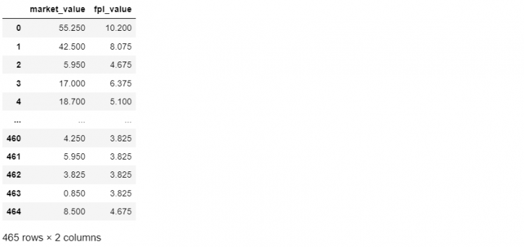

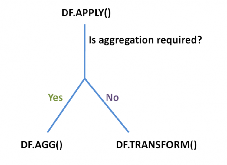
The apply Method in DataFrame

We use the apply method whenever we want to apply a given method to an entire DataFrame, a row or column at once.

For example, we wish to modify all our floating point columns and round them to the closest integer without actually converting them.

• STEP 1: We can start by defining a function round_floats, which will take a single parameter. Inside the function we will check the type of the variable, if it is a float we return the rounded version of that series, and if it isn’t we simply return the series unchanged.

def rounded_floats(x):
    if x.dtype == np.float64:
        return round(x)
    
    return x

• STEP 2: Applying rounded_floats function to all the float columns.

# Applying the rounded_floats function and using head method to print
df.select_dtypes(np.float64).apply(rounded_floats).head()

NOTE: The apply function is very similar to the transform method. The only difference is that the apply method is a bit more flexible since it supports aggregation as well as the same shape transform. The apply function is a combination of the transform method and the aggregate method.

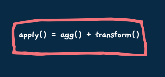
The apply function is very advanced and flexible and supports two kinds of operations.

• The ones that change the shape and dimensions of the underlying DataFrame, which would be the aggregate or the agg function.
• The ones that apply inplace transformations, that would identically return the same shape as that of the original DataFrame, which would be the transform function.

Now if we wanted to aggregate our numerical columns, the typical way of doing that is by using the agg method. But now we know that the apply method can also act as the agg method.

We could simply apply the following command to find out the mean across all columns of the DataFrame:

# Finding the mean using the apply function
df.apply('mean')

# Output
age              26.776344
position_cat      2.178495
...
club_id          10.253763
big_club          0.309677
new_signing       0.144086
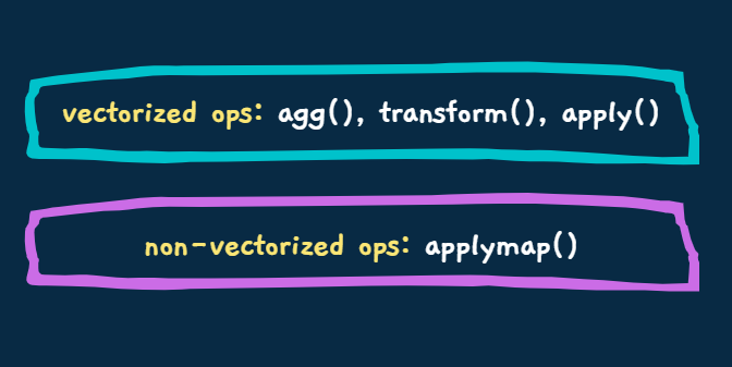
dtype: float64

Element-wise Operations with applymap()

The agg, transform, and apply methods operate on entire columns or rows at once. These take advantage of the concept of vectorized operations, which is a NumPy feature that allows us to realize huge performance gains by applying the given operation on a set of values all at once.

Occasionally we might be working on some function whose logic depends upon accepting and operating on an individual value, i.e. operating one item at a time. For such cases, Pandas offers the applymap function.

Let us take an example that we want to adjust our players’ market_value and the fpl_value for inflation (a general increase in the price). So we want to increase our market_value and fpl_value by 2%.

To make it more non-vectorized, let us assume we also want to know precisely when each 100th value was adjusted for inflation. So for every 100 values, we want the function to print out the timestamp for when the transformation took place.

• STEP 1: Since the values have to be appreciated by 2%, we will have to multiply our existing values by 1.02 therefore, saving it in a variable as inflation.

inflation = 1.02

• STEP 2: We will seperate the DataFrame slice we want to modify and store it in a seperate variable mini_df.

mini_df = df.loc[: , ['market_value', 'fpl_value'] ]

# Printing the DataFrame slice
print(mini_df)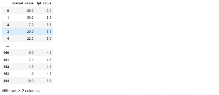

• STEP 3: Now we need to define our custom function as the log_and_transform which takes in a single parameter. We also set a counter to keep the track of every 100th element. Now increment the counter by 1, and if the counter is divisible by 100 we print the timestamp.

from datetime import datetime
counter = 0

def log_and_transform(x):
    global counter
    counter += 1
    if counter % 100 == 0:
        print(f"It's {datetime.now()} and I just adjusted the {counter}th value.")
    
    return x * inflation

• STEP 4: Now applying this log_and_transform function to our DataFrame slice mini_df.

mini_df.applymap(log_and_transform)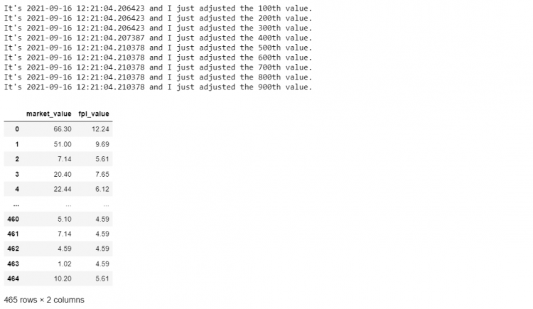

The log_and_transform function is impossible to vectorize without losing functionality. It only fulfills its functions when the values are passed one at a time.

Setting DataFrame Values

Sometimes we do not want a large-scale operation to transform the entire row or column at once. We just want to spot-change our data, to modify a single specific value. We can easily do this using the Assignment Operator (=).

Let us try to understand with the help of an example, suppose we want to change Theo Walcott’s position from RW to CM in our DataFrame.

Using label based indexing (loc)

We can do this by locating the element using the loc indexer and then using the assignment operator to set it to a new value.

# Assigning a new value using loc indexer
df.loc[3, 'position'] = 'CM'

Using position based indexing (iloc)

Another way of doing this is through position-based indexing using the iloc indexer.

# Assigning a new value using iloc indexer
df.iloc[3, 3] = 'CM'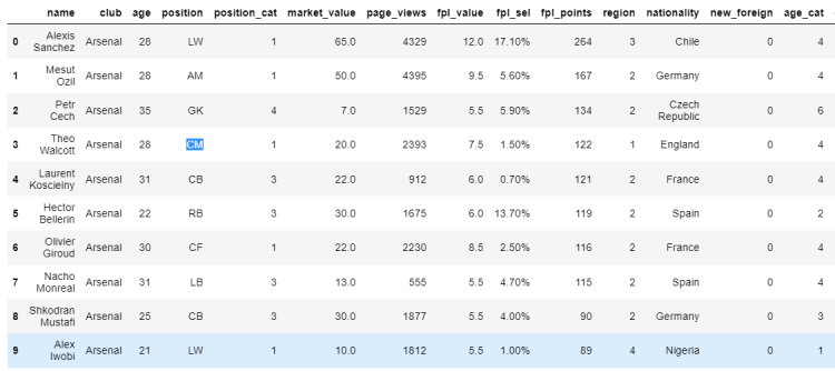

However, the at and iat indexers should be preferred for single-value assignments. The at and iat indexers support only one type of syntax and therefore have much less overhead in their function definitions. This means that at and iat indexers are extremely fast as compared to loc and iloc.

The SettingWithCopy Warning

Pandas may throw a warning when we try to update or set values in our DataFrames. This is encountered when we use a different approach to change values of elements, using the square bracket indexing method.

Now if we want to select a specific player’s page_views count, we can use another square bracket associated with his position in the DataFrame.

df['page_views']

# Output
0      4329
1      4395
2      1529
       ... 
463     412
464     214
Name: page_views, Length: 465, dtype: int64

Let us say we want to modify the page_views for the second index. Now that we’ve got the element to be updated, we can go ahead and assign it a new value.

df['page_views'][2] = 2001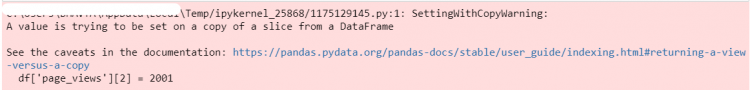

However, we get the following warning – “A value is trying to be set on a copy of a slice from a DataFrame.” The reason why we are getting this warning is that Pandas cannot guarantee that we are working with the actual underlying DataFrame when we do indexing like this (Chained indexing).

When using chained assignment, Pandas cannot determine whether we are working with a copy of the data or a view of the underlying DataFrame. If we are working with a copy of the DataFrame, changes made to its elements will not be reflected in the actual data.

Changes may or may not be reflected, based on the structure of how the memory is stored. But this is not guaranteed. Hence, we get the mentioned warning.

Let us check whether the changes that we made above happened in the actual DataFrame or not.

df.head()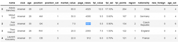

In this case, the changes we made can be seen in the actual underlying DataFrame. This indicates that we were working on its view, not a copy of the same.

Whenever performing an assignment when working with a copy of the DataFrame (like using the drop_dupicates() function), we will get the same warning message. Henceforth, no changes are applied to the original underlying data.

It is possible to turn off this warning manually by setting the chained assignment mode to none. The chained assignment mode in the options of Pandas is currently set to “warn”. We can set this to “None” to not get the warning message. However, it is considered good practice to consider the warning issued by Pandas.

pd.options.mode.chained_assignment = ‘None’

View vs Copy

Whenever we index, extract slices or apply a method to our DataFrame, we technically run into the question of whether we are working on the actual DataFrame or its copy.

Views in a DataFrame

A view is like a window into the underlying DataFrame. It gives us direct access to the data. We can update and modify the actual data when working with a view of the DataFrame.

Copies in a DataFrame

 A copy, on the other hand, is a replica of the actual data. It may or be the same as the original DataFrame. Any changes made to a copy will not be reflected in the underlying DataFrame.

The problem arises when we have to determine by ourselves when we are working a view of the DataFrame or a copy. This can be determined if we make use of the following 2-point rule:

• Pandas tends to give us copies of the DataFrame.
• If we use loc/iloc or at/iat, we are guaranteed to get a view.

Let us consider an example where we use the loc indexer to modify the elements of the DataFrame and see whether or not the changes appear in the actual data.

# Modifying elements of the DataFrame
df.loc[0:3, ‘position’] = [‘CM’, ‘RW’, ‘CB’, ‘GK’]

df.head()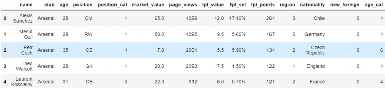

As we can see, the changes that we made in the view of the DataFrame were reflected in the underlying data.

In the above case, we used the iloc indexer for the DataFrame. Hence, we get a view of the DataFrame. However, if we use the same function on an attribute instead of the entire DataFrame, or some other function like drop_duplicates(), we will be breaking the rule.

In these cases, we will again receive the SettingWithCopy Warning from Pandas.

df['age'].iloc[1] = '12'

df.drop_duplicates().loc[3, 'position'] = 'CM'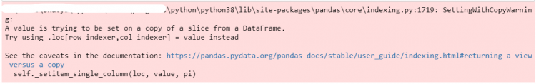

Adding DataFrame Columns

We sometimes feel the need to expand our data set by adding new attributes. Let us discuss a few methods to do so.

Using the assignment operator

The easiest and the most common approach to adding new columns is by using the assignment operator on square brackets with a label that doesn’t yet exist.

Let us say, we want to add a new column MVtoFPL in our original DataFrame. So we will confirm that the column name MVtoFPL does not already exist by using the following command.

'MVtoFPL' in df

# Output
False

Now, we can simply use MVtoFPL in square brackets and set it to a default value.

# Introducing a new column with a default value
df['MVtoFPL'] = 1.0

# Checking if 'MVtoFPL' exists in the DataFrame
'MVtoFPL' in df

# Output
False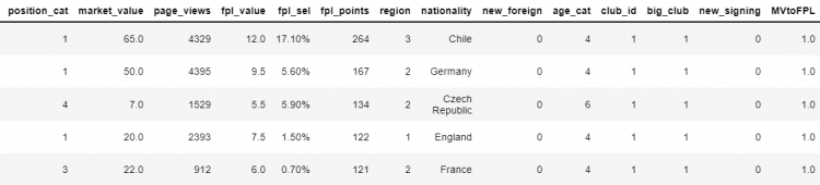

We can check towards the very end of the DataFrame, we see that the new attribute MVtoFPL is added.

Now, we need to update the value of this column to the ratio of market_value and fpl_value columns. The syntax is identical except now we’re setting it to a different value and not creating it.

# Setting the value of the new attribute
df['MVtoFPL'] = df['market_value'] / df['fpl_value']

df.head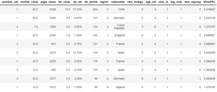

Using the insert method

Another method for inserting new columns in the DataFrame is by using the insert function.

Now for this example, let us slice our DataFrame and store it in a variable df_mini.

# Slicing our original DataFrame
df_mini = df.iloc[:4, 1:5]

Let us assume we are working with this DataFrame and we need to add a new attribute as the name of the player. We will start by creating a series that contains the names of the players and store them as player_names.

# Creating a series of player names
player_names = pd.Series(['Bronson', 'Bradley', 'Ronald', 'Ronny'])

print(player_names)

# Output
0    Bronson
1    Bradley
2     Ronald
3      Ronny
dtype: object

Now, we want to insert the new set of values into our mini DataFrame df_mini using the insert function.

df_mini.insert(0, 'nicknames', player_names)

print(df_mini)

The insert method not only allows us to add a new column but also lets us specify exactly at which position we want our new column to be placed. We are also able to provide a name to our column, which in this case is nicknames.

Using the assign method

The assign method assigns new columns to an existing DataFrame and returns a new copy.

Let us create a new column as career_goals for the total goals scored by the player in his career.

df_mini.assign(career_goals = [12, 67, 179, 49])

NOTE: We can also add multiple methods using the assign method which we couldn’t use the insert method. We can add multiple columns using the following approach.

df_mini.assign(
        career_goals = [12, 67, 179, 49], 
        nationality = ['American', 'British', 'Turkish', 'Indian']
)

Adding Rows to DataFrame

We may come across situations where we need to expand our DataFrame by adding more rows to the same. There are various methods for achieving this.

Using the append method

The first method that we will go through is the append method. The append method works with Series, DataFrames, or a collection of them.

Passing Series object as parameter

Before appending the DataFrame, let us create the following Series. We’ll name the Series ‘4’ for now.

cristiano = pd.Series({
    'nicknames' : 'Cristiano',
    'age' : 32,
    'position' : 'RW',
    'club' : 'Juventus',
    'position_cat' : 1
}, name = 4)

We can confirm whether or not the object was created accordingly.

print(cristiano)

# Output
nicknames       Cristiano
age                    32
position               RW
club             Juventus
position_cat            1
Name: 4, dtype: object

Now that we have created our Series object, we can use the append function to add this object to the required DataFrame. In the following example, we will use the append function on the df_mini DataFrame and pass the object ‘cristiano’ as a parameter.

df_mini.append(cristiano)

Running this program will yield a copy of the DataFrame that includes the newly added Series object in the rows. The name of the Series we previously created becomes the index label for the appended row.

Passing list of Series objects as parameters

Furthermore, the append method also supports adding multiple Series objects at once to the DataFrame. For this, we need to create multiple Series objects and pass them as a list in the parameter for the function.

df_mini.append(player_1, player_2, player_3,…)

Passing DataFrame object as parameter

Instead of using the above way, we can create a DataFrame object. This object will hold the values of several players as lists simultaneously. Let us consider the following examples.

other_players = pd.DataFrame({
    'nicknames' : ['Gianluigi', 'Lionel'],
    'age' : [37, 32],
    'position' : ['GK', 'CF'],
    'club' : ['Juventus', 'Barcelona'],
    'position_cat' : [4,2]
}, index = [5, 6])

Henceforth, we can confirm whether or not the object was created.

print(other_players)

Now that we have created our DataFrame object, we can use the append function to add this object to df_mini. In the following example, we will use the append function on the df_mini DataFrame and pass the object ‘other_players’ as a parameter.

df_mini.append(other_players)

Using the loc/iloc indexers

This is another technique that we can use to add new rows to our existing DataFrame. We can accomplish this by simply assigning a value to a loc or iloc view.

In the following example, we will assign a value to a specific index in the loc indexer. The data to be added will be passed as a list.

df_mini.loc[9] = ['Ramos', 'PSG', 35, 'CB', 4]

We can confirm if the new row has been added or not by running the following command.

print(df_mini)