Computational Photography refers to digital image capture and processing techniques that use digital computation instead of optical processes. Computational photography can improve the capabilities of a camera, or introduce features that were not possible at all with film-based photography, or reduce the cost or size of camera elements.
Examples of computational photography include in-camera computation of digital panoramas, high dynamic-range images, and light field cameras.
OpenCV provides different computational photography techniques such as Image Denoising, Image Inpainting, High dynamic range.
Image Denoising
Earlier, we have seen many image smoothing techniques like Gaussian Blurring, Median Blurring, etc and they were good to some extent in removing small quantities of noise.
Previously, we took a small neighborhood around a pixel and did some operations like Gaussian weighted average, a median of the values, etc to replace the central element.
In short, noise removal at a pixel was local to its neighborhood. There is a property of noise. Noise is generally considered to be a random variable with zero mean.
Consider a noisy pixel, p= p1+ n, where p1 is the true value of the pixel and n is the noise in that pixel. If we consider a large number of the same pixels( N ) from different images and compute their average, we should get p= p1 since the mean of the noise is zero.
We need a set of similar images to average out the noise. Consider a small window (say 5×5 window) in the image. Chance is large that the same patch maybe somewhere else in the image. Sometimes in a small neighborhood around it. We are using these similar patches together and find their average.
The blue patches in the image look similar. Green patches look similar. So we take a pixel, take a small window around it, search for similar windows in the image, average all the windows and replace the pixel with the result we got. This method is Non-Local Means Denoising.
Non-Local Means Denoising takes more time compared to the blurring techniques we saw earlier, but its result is very good.
OpenCV provides four variations of this technique. They are:-
- FastNIMeansDenoising – works with single grayscale images
- FastNIMeansDenoisingColored – works with a color image.
- FastNIMeansDenoisingMulti – works with image sequence captured in a short period of time (grayscale images)
- FastNIMeansDenoisingColoredMulti – works with image sequence captured in a short period of time, but for colored images
Common Parameters
- h: parameter deciding filter strength. A higher h value removes noise better but removes details of the image also. (10 is ok)
- h For Color Components: same as h, but for color images only. (normally same as h)
- templateWindowSize: should be odd. (recommended 7)
- Search window size: should be odd. (recommended 21)
FastNIMeansDenoising()
Perform image denoising using a Non-local Means Denoising algorithm with several computational optimizations. Noise is expected to be a gaussian white noise.
Parameters
- src – Input 8-bit 1-channel
- Dst – Output image with the same size and type as src
- h-luminance – Parameter regulating filter strength. Big h value perfectly removes noise but also removes image details, smaller h value preserves details but also preserves some noise
- Template window size – Size in pixels of the template patch that is used to compute weights. Should be odd. Recommended value 7 pixels
- Search Window size – Size in pixels of the window that is used to compute weighted average. Should be odd. Greater search window size – greater denoising time. Recommended value 21 pixels
import numpy as np
import cv2 as cv
from matplotlib import pyplot as plt
img = cv.imread('C:\images\noisy-1.jpg')
dst = cv.fastNlMeansDenoising(img,None,15,7,21)
plt.subplot(121),plt.imshow(img)
plt.subplot(122),plt.imshow(dst)
plt.show()
FastNIMeansDenoisingColored()
The function converts the image to CIELAB colorspace and then separately denoises L and AB components with given h parameters using the fastNlMeansDenoising function.
Parameters
- src – Input 8-bit 3-channel image
- Dst – Output image with the same size and type as src
- H – Parameter regulating filter strength for the luminance component
- H color – The same as h but for color components. For most images value equals 10 will be enough to remove colored noise and do not distort colors
- Template Window size – Size in pixels of the template patch that is used to compute weights. Should be odd
- Search Window size – Size in pixels of the window that is used to compute weighted average for given pixel. Should be odd
import numpy as np
import cv2 as cv
from matplotlib import pyplot as plt
img = cv.imread('C:\images\noisy-2.png')
dst = cv.fastNlMeansDenoisingColored(img,None,15, 15,11,17)
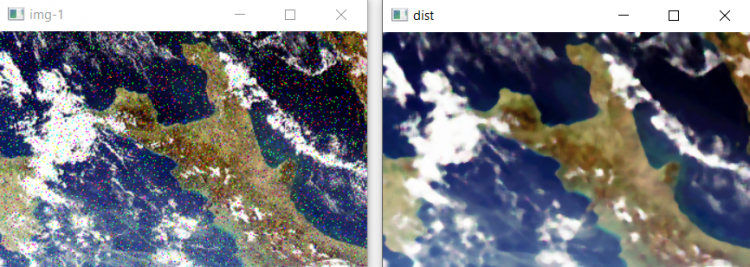
cv.imshow('img-1', img)
cv.imshow('dist', dst)
In the below figure we can notice a reduction of noise in the resulting image and the source image. We can try to alter the values of h, template, and search window sizes for better results.

High Dynamic Range
High-dynamic-range imaging is a technique used in imaging and photography to reproduce a greater dynamic range of luminosity than is possible with standard digital imaging. While the human eye can adjust to a wide range of light conditions, most imaging devices use 8-bits per channel, so we are limited to only 256 levels.
When we take photographs of a real-world scene, bright regions may be overexposed, while the dark ones may be underexposed, so we can’t capture all details using a single exposure. HDR imaging works with images that use more than 8 bits per channel allowing a much wider dynamic range.
There are different ways to obtain HDR images, but the most common algorithms are Debevec, Robertson used to generate and display HDR images from an exposure sequence, and demonstrate an alternative approach called exposure fusion (Mertens).
The main difference between the Debevec, Robertson, and Mertens approach of constructing an HDR image is, Mertens, does not require the exposure times data.
Steps for processing High Dynamic Range images:-
- Loading the list of different exposures of a single image
- Storing the exposure times of respective images
- Merge exposure sequence into one HDR image
- Converting HDR image back to 8-bit image ( Tone mapping )
Loading exposure images and their exposure times into a list
import cv2 as cv
import numpy as np

img_fn = ["C:\images\pic-1.png", "C:\images\pic-2.png", "C:\images\pic-3.png"]
img_list = [cv.imread(fn) for fn in img_fn]
exposure_times = np.array([15.0, 2.5, 0.25, 0.0333], dtype=np.float32)
Merging exposures using Debevec and Robertson
merge_debevec = cv.createMergeDebevec()
hdr_debevec = merge_debevec.process(img_list, times=exposure_times.copy())
merge_robertson = cv.createMergeRobertson()
hdr_robertson = merge_robertson.process(img_list, times=exposure_times.copy())
Tonemapping HDR images
We map the 32-bit float HDR data into the range [0..1].
tonemap1 = cv.createTonemap(gamma=2.2)
res_debevec = tonemap1.process(hdr_debevec.copy())
res_robertson = tonemap1.process(hdr_robertson.copy())
Convert to 8-bit and saving
In order to save or display the results, we need to convert the data into 8-bit integers in the range of [0..255].
res_debevec_8bit = np.clip(res_debevec*255, 0, 255).astype('uint8')
res_robertson_8bit = np.clip(res_robertson*255, 0, 255).astype('uint8')
Debevec
Robertson
Merge exposure sequence using Mertens fusion
Using Mertens fusion we dont need exposure times and need not apply tone mapping because Mertens fusion already gives us the values between [0,1].
Once the images are merged we need to convert them into 8-bit images to display them.
import cv2 as cv
import numpy as np


img_fn = ["C:\images\pic-1.png", "C:\images\pic-2.png", "C:\images\pic-3.png"]
img_list = [cv.imread(fn) for fn in img_fn]
merge_mertens = cv.createMergeMertens()
res_mertens = merge_mertens.process(img_list)
res_mertens_8bit = np.clip(res_mertens*255, 0, 255).astype('uint8')
As we can notice the result of merging the different exposure images and the ease of implementation is much better compared to Robertson and debevec.

Image Inpainting
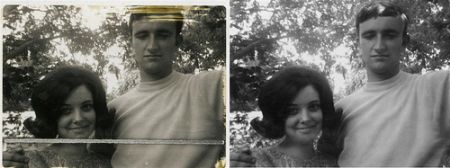
Most of us will have some old degraded photos at our home with some black spots, some strokes, etc on them. For restoring it back we can’t simply erase them in a paint tool because it is will simply replace black structures with white structures which is of no use. In these cases, a technique called image inpainting is used.
The basic idea is simple: Replace those bad marks with its neighboring pixels so that it looks like the neighborhood.

Several algorithms were designed for this purpose and OpenCV provides two of them. Both can be accessed by the same function, cv2.inpaint().
The first algorithm is based on the paper An Image Inpainting Technique Based on the Fast Marching Method by Alexandru Telea in 2004. It is based on the Fast Marching Method.
The algorithm starts from the boundary of this region and goes inside the region gradually filling everything in the boundary first. It takes a small neighborhood around the pixel on the neighborhood to be inpainted. This pixel is replaced by the normalized weighted sum of all the known pixels in the neighborhood.
FMM ensures those pixels near the known pixels are inpainted first so that it just works like a manual heuristic operation. This algorithm is enabled by using the flag, cv2.INPAINT_TELEA.
The second algorithm is based on the paper Navier-Stokes, Fluid Dynamics, and Image and Video Inpainting by Bertalmio, Marcelo, Andrea L. Bertozzi, and Guillermo Sapiro in 2001. This algorithm is based on fluid dynamics and utilizes partial differential equations.
It first travels along the edges from known regions to unknown regions. It continues isophotes (lines joining points with the same intensity, just like contours joins points with the same elevation) while matching gradient vectors at the boundary of the inpainting region. This algorithm is enabled by using the flag, cv2.INPAINT_NS.
cv2.inpaint(src, mask, inpaintRadius, flag)Parameters
- src – Input 8-bit, or 8-bit 3-channel image
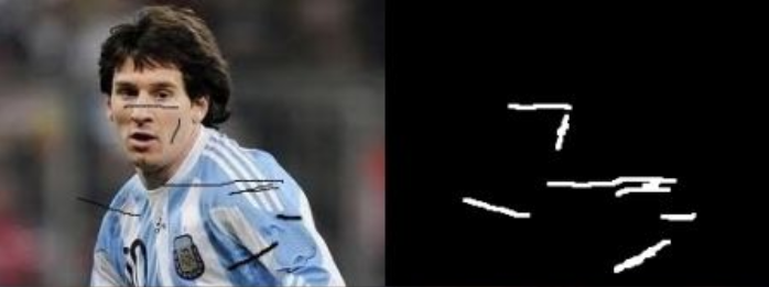
- mask – Inpainting mask, 8-bit 1-channel image. Non-zero pixels indicate the area that needs to be inpainted
- inpaintRadius – Radius of a circular neighborhood of each point inpainted that is considered by the algorithm
- flag – Inpainting method that could be either
cv2.INPAINT_TELEAorcv2.INPAINT_NS
The next step is to create a mask of the same size as that of the input image, where non-zero pixels correspond to the area which is to be inpainted. We created a corresponding stroke with the Paint tool.

import numpy as np
import cv2 as cv
img = cv.imread('messi_2.jpg')
mask = cv.imread('mask2.png',0)
dst = cv.inpaint(img,mask,3,cv.INPAINT_TELEA)
cv.imshow('dst',dst)
cv.waitKey(0)
cv.destroyAllWindows()
