In previous articles, we mainly focused on Artificial Neural Networks and Convolutional Neural Networks for solving problems in NLP. In this article, we will get an introduction to Recurrent Neural Networks.
In ANNs, we had seen that it is a network where the inputs are independent of one another and we build a network with stacks of layers that help us achieve better performance. In CNN’s, we had seen that we try to find the spatial relationships between input data.
Recurrent Neural Networks
First, let’s make it clear that Recurrent Neural Networks are a type of artificial neural network. RNNs are extensively used in NLP due to their working and usefulness in the context of NLP.
The basic idea of an RNN is that it provides a sense of memory which is essential for superior NLP performance. Unlike other networks, the inputs to the RNN aren’t independent of each other. RNNs help to recognize patterns in a sequence of data.
We’ll look into the working of an RNN in-depth later, but first, let’s understand how they are useful for NLP.
Why are they extensively used in NLP?
As we saw in the definition of RNNs, they are neural networks that help recognize patterns in a sequence of data. A lot of different types of data can be a sequence of data. But if we focus on text data, we see that text data itself is a sequence or a sequential type dataset.
When we read the text we read it from left to right (in English). There is a flow between the words and phrases. There is a sequence. Consider the following example.
It was cloudy yesterday so it might rain today. In the sentence, we see that there is a sequence in the text. Some words in a text may be influenced i.e. affected by words from previous sentences. Some texts may have words that are influenced by words present in various sentences. Getting the context is necessary.
Hence when RNNs are used, they add a sense of memory to the text. And with the help of this memory, RNNs can find the sequential relationship between words in different sentences.
With the help of RNNs, we can better understand the context of the sentences and this will help us make predictions with the text. Now that we have a little knowledge about how RNNs can be beneficial for NLP, we’ll look at the structure of an RNN.
RNN architecture
Now, let’s focus our attention on the architecture of the Recurrent Neural Network. If you look at the image shown below, you can observe the actual structure of an RNN.
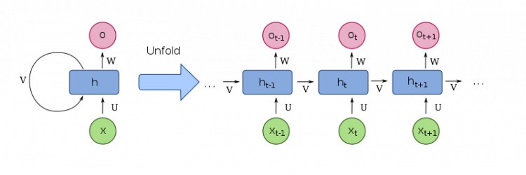
The left part of the image shows the RNN architecture of a single RNN neuron. If you recall, a neuron is the main building block of any neural network. The left part in the image is a single RNN neuron representation.
Remember, every neuron in an RNN takes in two inputs, one input we provide externally and the other one we don’t explicitly provide. The second input is called the hidden state. It’s called a hidden state because this type of input is not provided by us and is thus hidden to us.
In the image, the neuron has an input and output. Suppose for a time state say “t” i.e. we consider a time period, we provide input to the neuron “x” and we see that this input enters the neuron and this is denoted by “U”.
The input is then processed by the neuron, but you notice another input is denoted by “V”. We ourselves are not providing this input then where is it coming from? It is coming from a previous time state. This is the hidden state input and is provided by the neuron from the previous time step.
We also notice the output process denoted by “W”. When we unfold this neuron i.e. we expand the working of the neuron in different time steps, get the right part of the image. Three time steps are shown in the right part. One is the past, the second is the present and the third is the future step.
“ht” denotes the present step, “ht-1” denotes the past, and “ht+1” denotes the future step. Remember that these are not three different neurons but the same neuron in different time states. Notice that as time progresses, the hidden state input “V” is also passed on from one state to another along with the inputs we provide.
We have now a better understanding of how an RNN works.
Comparison to an ANN
We now compare the Recurrent Neural Network with an Artificial Neural Network to better understand the RNN.
The main difference between the ANN and RNN is that in ANN the inputs were independent of each other. In ANN, we used to provide the inputs and only those inputs were taken into consideration when the model had to predict anything.
This is different in RNN where the inputs are linked to each other through time. The inputs are connected through time. Take a look at the image below. The image shows the RNN and each circle in the rectangular box is the neural network.
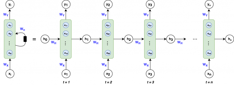
As you can see, the Recurrent Neural Network is unfolded through time and the input from the previous state is passed to the current time state. Again, remember that this is a single RNN only, not three RNNs.
An ANN is not unfolded through time, but it gets only a single input i.e. the input we provide and that input is then forwarded to different layers before it reaches the output layer. Whereas in RNN, as we saw, there are two inputs and the layers are linked to each other through time steps.
The image shows a many to many RNN. This means that the many to many RNN takes several inputs and outputs several outputs at once. This type of RNN is very useful for music and lyrics generation among other things.
Forward propagation in RNN
Now, we’ll see how forward propagation takes place in the Recurrent Neural Network. Forward propagation is basically the process of propagating the input data from the input layers towards the output layers.
To help you visualize forward propagation think of the data entering the network from left and exiting through right as output. So the word “forward” in forward propagation means that the data is traveling from the input layers to the output layers in a forward sense.
In RNN, forward propagation means the two inputs we had discussed previously i.e. the input we provide and the hidden state input are used as inputs at a particular time state and the output is carried forward as the hidden state input to the next time state along with an external input.
So, at one time step, the model will have two inputs (one by us and the second being the hidden state) and after processing, its output will be used as hidden state input in the next time step. This is how forward propagation works in an RNN.
Backpropagation
In the previous section we had seen forward propagation in RNN, now we’ll focus on backward or backpropagation. As the name suggests, it is exactly the opposite to forward propagation.
In forward propagation, we had seen that data travels from the input towards the output direction but in backpropagation, data travels from the output direction towards the input direction. Look at the image below. It shows backpropagation and forward propagation in a network.
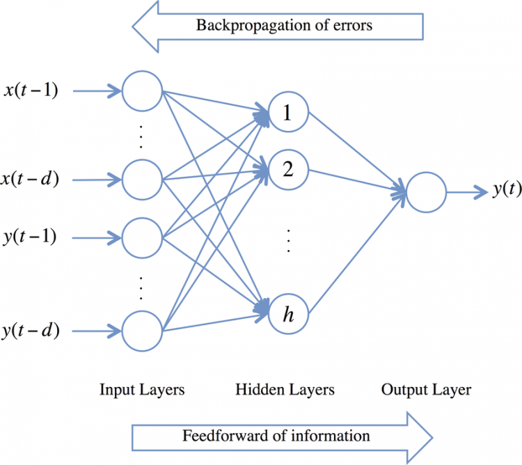
You can see the errors are being backpropagated in the image. And the direction is from the output towards the input of the network. Every network gives an output. It may be a regression output (a number) or a class label (classification).
The model compares this output to the actual true value also called the ground truth and it sees how correct or how wrong its predicted output was when compared to the ground truth. This is the error calculation.
And based on this, the model tries to update its weight parameters in the model by sending back the error so that next time model may perform better and gives a more accurate output. This updation of weights is done through a process called backpropagation.
Backpropagation Through Time (BPTT) in RNNs
In the previous section, we have seen what backpropagation is how it is done. In RNNs backpropagation is done a bit differently. The errors are not just sent back like in an ANN because RNNs are trained through time steps and thus the errors too must be backpropagated through the time steps.
As we know, RNNs consider time steps for calculating the final output. We have seen that the hidden state input is propagated from one time step to the next. Note that across different time steps the neurons are the same it’s just that they fire differently for different time steps.
In backpropagation in RNN, the error calculated is sent back through the time steps. Each time is dependent on the previous time step for computation. So the error must be sent back through time along the same neuron.
To backpropagate efficiently we calculate the gradient of the parameters that contributed to the final output calculation. In ANNs, when we are backpropagating, we calculate the gradient for different layers but in RNNs we backpropagate through time for the same layer. The layers give a different output with each time step.
Refer to the image given below. It shows the backpropagation process in an RNN. Refer to it as we go through the explanation and it will help you understand this process better.
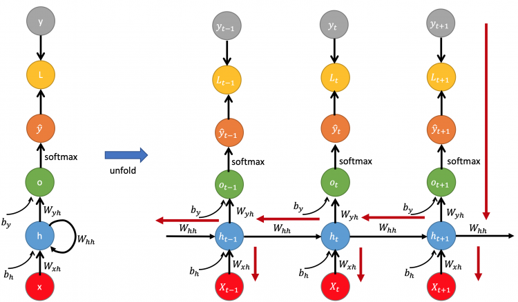
The image shows backpropagation through time. When we unfold the network on the left, we get the unfolded version of the network in time on the right. It shows three time steps. You can see the error is propagated back through the red line.
First, the error is propagated through the most recent parameters and the gradient is calculated for that parameter. Then, it travels backward in time and the error reached the previous time step. This is how it was trained and forward propagated and this is the same path it follows backward.
One thing to note here is that the weights Whh are constant even through time in the forward sense. And thus, when backpropagating, we aggregate the weights and gradients and then apply them once only rather than updating each parameter separately. Because that is not it was trained.
Vanishing gradient problem in RNNs
This is one of the main problems faced by the RNNs. Let’s try to understand what causes this problem and what options we have to reduce the severity of this problem.
RNNs are neural networks that are trained through the use of backpropagation of errors. Our main aim is to minimize the cost function (predicted value – actual value) and for this we use gradient descent to find the global minimum.
If you recall, as we discussed in previous sections, for the final out calculation every neuron in the previous time step has contributed to the training of the future neurons. This is how RNNs work and learn. This is where the problem arises. The RNN is very deep and has many layers when training through time.
Due to this, when the errors are backpropagated through the layers through time, due to so many layers what happens is that the gradients (derivatives of the weights w.r.t. error function) systematically keep on decreasing to the point that they vanish. This is called the vanishing gradient problem.
The result of this problem is that the training of the model may stop completely due to weights not getting updated at all. Because weight updation depends on the gradients being calculated for that weight. As gradients vanish i.e. diminish the training may stop and this leads to poor performance of the network.
Steps to mitigate the vanishing gradient problem:
- Initialize weights so that the potential for vanishing gradients in minimized.
- Have Echo State Networks that are designed to solve the vanishing gradient problem.
- Have Long Short-Term Memory networks (LSTMs).
Exploding gradient problem in RNNs
The exploding gradient problem is just the opposite of what we have seen in the vanishing gradient problem.
In exploding gradient problem, the gradients that are calculated are increasing i.e. exploding as we go deeper through the layers. This is in contrast to the vanishing gradient problem where the gradients are diminishing.
Gradients are of utmost importance when adjusting the weights of the network. Weights need to be adjusted so that the cost function is minimized because only when the cost function is minimized, our model will perform with more accuracy.
It all comes down to the gradients. If the gradients are minimized and are vanishing with each subsequent layer in time then it gives rise to the vanishing gradient problem, whereas if the gradients keep on increasing i.e. exploding then it gives rise to the exploding gradients problem.
Steps to overcome the exploding gradients problem:
- Stop backpropagating after a certain point although this is not always optimal because not all of the weights get updated.
- Penalize the gradients or artificially reduce gradient.
- Perform gradient clipping i.e. put a maximum limit on the value of the gradient.
Multiple forms of RNNs
In this final section on RNNs, we will take a look at the different ways an RNN network can be arranged to provide input and get the output.
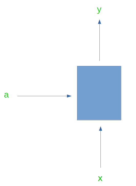
One-to-one
In this form of the RNN, the RNN takes a single input and provides a single output. This is the simplest form the RNN can take. One-to-one RNN is shown in the image below.
One-to-many
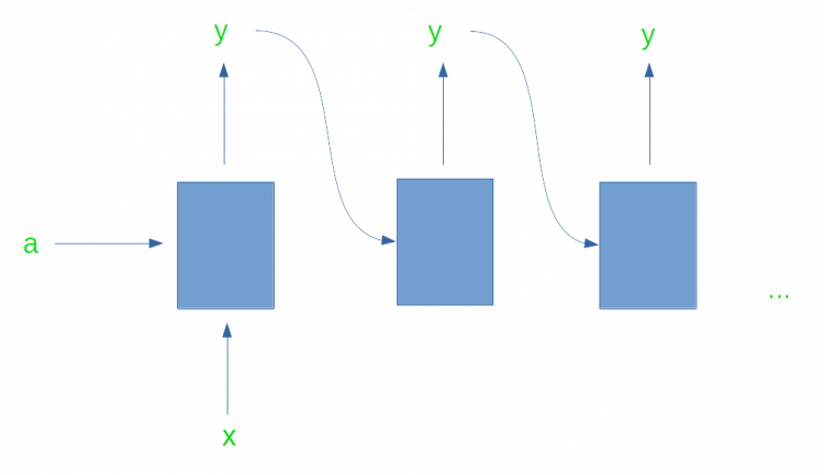
In this form of RNN, the network takes in a single input and produces multiple outputs. Hence it is called one-to-many. One example where such an RNN is used is for music generation.
In music generation, a single note is given as an input to this form of RNN and the RNN generates music based on that note.
The one-to-many form of an RNN is shown below.
Many-to-one
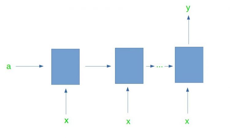
This form of the RNN, as the name suggests, takes in multiple inputs at a time and produces a single output. This form of RNN finds applications in tasks such as sentiment analysis.
In sentiment analysis, multiple words are fed into the network, and the network processes and outputs a single output stating the sentiment of the text.
This form of the RNN is shown in the image below.
Many-to-many
These RNNs take in multiple inputs and produce multiple outputs. These types of RNN are further subdivided into two forms. The further division is based on whether the size of the inputs is equal to or not equal to the size of the output.
Tx = Ty
This is the many-to-many form in which the input is equal to the output. This form of the RNN is used in Named Entity Recognition (NER).

Tx != Ty
This is the many-to-many form in which the size of the input is not equal to the size of the output. The application of this form is found in Machine Translation. This form can easily produce output greater than or less than the size of the input string.

Final thoughts
In this article, we have been introduced to Recurrent Neural Networks. We saw its basic architecture, we saw how information is forward propagated and backward propagated. Then we went over two problems faced by RNNs i.e. vanishing and exploding gradients and finally we covered different forms of RNNs.
