In the ’90s to perform complex operations the most powerful algorithm available is Support Vector Machines ( SVM ). Back then there was no sufficient computational power. Since 2006 several algorithms are developed for training neural networks. Among those algorithms, CNN is one of them.
Convolutional Neural Network ( CNN ) is a deep learning algorithm that is commonly used in image classification. It takes an input image and assigns weights to different objects in the image and classifies them.
For classifying the images CNN uses different pre-built libraries such as TensorFlow, Keras, Matplotlib, seaborn, NumPy, etc.,
What is Tensorflow
TensorFlow is a free and open-source software library for machine learning. it can be used across a range of tasks but has a particular focus on the training and inference of deep neural networks.
Previously there aren’t many libraries that can create multiple layers in large-scale neural networks. But after Google releasing TensorFlow in 2015 and the updated version in 2019 performing classification, predictions, Discovering, Creation, Understanding has become a lot more efficient and easier.
Convolutional Neural Networks
Traditional Neural Networks create exactly a single neuron for handling a single pixel of an image in the input layer. If we consider there are n number of pixels in the image then there will be n number of neurons in the input layer which cannot be an efficient way of processing the neurons. This is where we use CNN to optimize the number of pixels.
Convolutional Neural Networks reduce the number of neurons in the input layer by removing unnecessary pixels in the image that don’t represent any useful information.
Benefits of using CNN:-
- It doesnot use all the pixels of the image
- It applies a dense neural network but at the beginning it transforms the Data
- It uses only the important feature of the image for feeding the input layer
Steps involved in transforming the data by CNN:-
- Feature Detector:- Feature detector is matrix containig 0’s and 1’s that is used to multiply with the corresponding matrix in the image. It provides feature map as output.
- Feature Map:- Feature Map consists of all the important pixels that are useful by the neural network. Feature map visualization will provide insight into the internal representations for specific input for each of the Convolutional layers in the model.
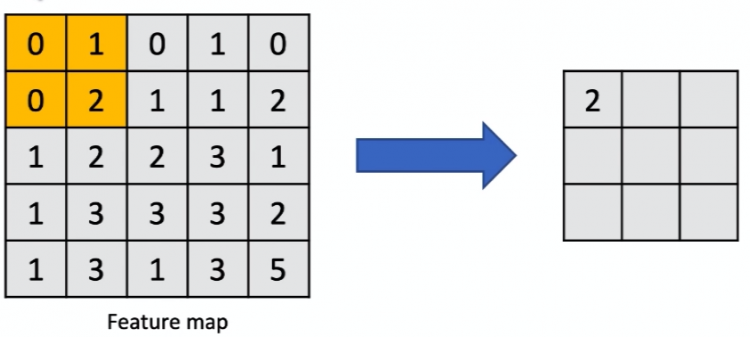
- Max Pooling:- Max pooling is the process of obtaining the value of maximum intensity in a particualr region by applying filter. Max pool is obtained by applying the relu function on all the matrix values present in Feature Map. All the values are fed into Max pool matrix
- Flattening:- Flattening is representing the matrix values of max pool in the form of a vector that can be fed for the first layer or input layer of the neural network.
The image below represents an image that is converted into a set of feature maps and then obtaining the Max pool of each of the feature maps. The maximum of the max pool is being converted into a vector of values to be fed as pixel values into the input layer.

Building and Evaluating CNN for Image Classification
We are using google collab which comes as a readily available jupyter notebook that has all the pre-built libraries necessary for evaluating the model.
Importing Libraries
import tensorflow as tf
from tensorflow.keras.models import Sequential
from tensorflow.keras.layers import Conv2D, MaxPooling2D, Flatten, Dense
from tensorflow.keras.preprocessing.image import ImageDataGenerator
import matplotlib.pyplot as plt
import seaborn as sns
import zipfile
import numpy as np
import cv2
from google.colab.patches import cv2_imshow
Loading Dataset
You can download the Dataset zip file from the link provided — Dataset
Once the Dataset is uploaded into your google drive you can mount the drive to your collab notebook.
from google.colab import drive
drive.mount('/content/drive')
After mounting the drive we can extract the zip file into the root location using zipfile module.
Note:- Path could be different because the google account connected varies from person to person and the location they store might be varying.
In case if the dataset you are working on is different, for loading that dataset into the model you need to perform data pre-processing. You can check out the face recognition tutorial where we performed the data processing technique
path = '/content/drive/MyDrive/homer_bart_2.zip'
zip_object = zipfile.ZipFile(file=path, mode='r')
zip_object.extractall('./')
zip_object.close()
Train and Test Dataset
We can configure some parameters to make modifications to the original images, which is very useful when we have few images of each class.
You can use ImageDataGenerator() for pre-processing the data and it also allows you to augment your images in real-time when the model is still training. You can perform transformations on each image while the image is being passed into the model. Parameters such as rescale, horizontal flip, zoom, rotation_range can be used.
training_generator = ImageDataGenerator(rescale=1./255,
                                        rotation_range=7,
                                        horizontal_flip=True,
                                        zoom_range=0.2)
Since the Training generator has been developed we can load the training data and define the number of classes the training data has been categorized into using the ‘class_mode’ parameter, and the number of images the neural network can consider at a time for training using the parameter ‘batch_size’.
For the model not to recognize the pattern of training the images and to avoid false predictions, we can apply shuffle = True.
train_dataset = training_generator.flow_from_directory('/content/homer_bart_2/training_set',
                                                        target_size = (64, 64),
                                                        batch_size = 8,
                                                        class_mode = 'categorical',
                                                       shuffle = True)
Printing the normalized dataset and the number of classes available in the dataset.

The same process follows for defining and loading the Test dataset, Except we don’t pass more parameters to ImageDataGenerator() of test_generator so that model couldn’t relate the data to the Train dataset.
test_generator = ImageDataGenerator(rescale=1./255)
test_dataset = test_generator.flow_from_directory('/content/homer_bart_2/test_set',
                                                     target_size = (64, 64),
                                                     batch_size = 1,
                                                     class_mode = 'categorical',
                                                     shuffle = False)
Building and Training the neural network
Building a CNN network is similar to the traditional neural network except for the part of adding a convolution layer for the input data. The first step involves applying a feature map, max-pooling, flattening concepts to obtain useful information of the image.
Since the Network is having a sequence of layers we can instantiate the Sequence class using Sequential(). For adding a layer we can use network.add().
Since the image we recognize is in the form of the 2-Dimensional matrix we use Conv2D(feature_maps, Kernel_size, input_shape, activation_function) and the parameters we can pass are:-
fetaure_mapsthe number of feature maps we define from the original image, by default we can assign this value to be 32Kernel_sizeis the matrix size of the feature detector that we apply on the image to obtain feature mapinput_shapeis the size of the image that we are using, since we redefined the shape to be 64×64 in the test and train dataset we use the same over hereactivation_functionwe apply in our network is the relu function to achieve a max-pooling matrix
Once the feature map is adding to the network the next step is to obtain a max pool with a pool size of (2, 2). We use MaxPooling2D().
In the below figure we apply a (2, 2) pool size on the feature map to get a maximum value in the applied area and store the value in the max-pool matrix.

network = Sequential()
network.add(Conv2D(32, (3,3), input_shape = (64,64,3), activation='relu'))
network.add(MaxPooling2D(pool_size=(2,2)))
We can keep on adding the layers till we build an efficient neural network, for classifying images. In our example, we apply the convolution layer 3 times to achieve better results.
Note:- The number of times the convolutional layer is defined depends on the test results and the predicting capability of the model, as per my experimental analysis I defined it for 3 times.
The next step would be to add the Flatten layer that converts the data in the max-pool into a vector. We use Flatten() for this purpose.
Since the input layer is built we define two hidden layers and a final output layer. In the output layer, we need two units since the model compares the images to classify between the two classes.
network = Sequential()

$adding convolutional layers
network.add(Conv2D(32, (3,3), input_shape = (64,64,3), activation='relu'))
network.add(MaxPooling2D(pool_size=(2,2)))

network.add(Conv2D(32, (3,3), activation='relu'))
network.add(MaxPooling2D(pool_size=(2,2)))

network.add(Conv2D(32, (3,3), activation='relu'))
network.add(MaxPooling2D(pool_size=(2,2)))


network.add(Flatten())

#hidden layers
network.add(Dense(units = 3137, activation='relu'))
network.add(Dense(units = 3137, activation='relu'))

#output layer
network.add(Dense(units = 2, activation='softmax'))
Once the neural network is built we can get the summary of all the data it is handling internally using the Summary() class.
network.summary()Model: "sequential"
_________________________________________________________________
Layer (type) Output Shape Param #
=================================================================
conv2d (Conv2D) (None, 62, 62, 32) 896
_________________________________________________________________
max_pooling2d (MaxPooling2D) (None, 31, 31, 32) 0
_________________________________________________________________
conv2d_1 (Conv2D) (None, 29, 29, 32) 9248
_________________________________________________________________
max_pooling2d_1 (MaxPooling2 (None, 14, 14, 32) 0
_________________________________________________________________
conv2d_2 (Conv2D) (None, 12, 12, 32) 9248
_________________________________________________________________
max_pooling2d_2 (MaxPooling2 (None, 6, 6, 32) 0
_________________________________________________________________
flatten (Flatten) (None, 1152) 0
_________________________________________________________________
dense (Dense) (None, 3137) 3616961
_________________________________________________________________
dense_1 (Dense) (None, 3137) 9843906
_________________________________________________________________
dense_2 (Dense) (None, 2) 6276
=================================================================
Total params: 13,486,535
Trainable params: 13,486,535
Non-trainable params: 0Now the Network is completely ready and can be trained on the dataset on which it is meant to classify the predictions. Before training the network we need to compile it on few parameters such as optimizer, loss, and metrics. These parameters are completely based on the network we build and the data we handle.
network.compile(optimizer='Adam', loss='categorical_crossentropy', metrics = ['accuracy'])The final step involves training the neural network on the train_dataset. An important point to notice here is the number of times we train the model on the dataset the more accuracy it gains by the end of the training.
For the purpose of training the network on the same dataset we apply epochs = 50 such that it runs over the same dataset 50 times and by the end of the training it reduces the loss and gains accuracy when compared over test_dataset.
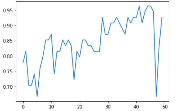
history = network.fit_generator(train_dataset, epochs=50, validation_data=test_dataset)Over here during the first epoch, the val_accuracy which determines the accuracy level is only 51% and by the end of the training, the accuracy level is reached is 92%.


Evaluating the Network
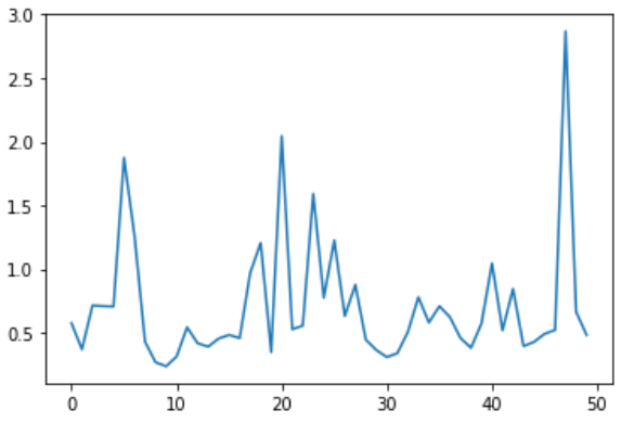
Evaluating the Network involves analyzing the test result when the network is trained over test_dataset. We also can draw a plot of the loss function and accuracy function as how they are at the start of training and also by the end of the training.
history.history.keys()# these are the key and value pairs stored in the history variable after training the network
# we can use these values to plot the loss and accuracy functions
dict_keys(['loss', 'accuracy', 'val_loss', 'val_accuracy'])plt.plot(history.history['val_loss']);
plt.plot(history.history['val_accuracy']);
Loss Function 
Accuracy Function
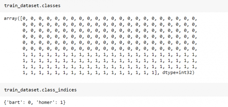
While training the model we have created two nodes on the output layer, which means the network analyzes the image and classifies the predicting score into two classes. We can also see the classes in the test_dataset.
test_dataset.class_indices{'bart': 0, 'homer': 1}In the predictions list if the first node value is higher than the second node it means the test image belongs to class 0 i.e., Bart. If the second node value is higher than the first node it means the image belongs to class 1 i.e., homer.
# predictions values range between 0 and 1
predictions = network.predict(test_dataset)
predictions
array([[1.00000000e+00, 3.50932505e-24],
[1.00000000e+00, 6.52031156e-18],
[7.84075141e-01, 2.15924904e-01],
..............................
............................
[1.81834592e-04, 9.99818146e-01],
[1.08367085e-01, 8.91632915e-01],
[2.29500259e-08, 1.00000000e+00]], dtype=float32)We can normalize the prediction values to be either 0 or 1 thus it resembles the classes 0 and 1 and compare the value with test_dataset.
predictions = np.argmax(predictions, axis = 1)
print(predictions)
print(test_dataset.classes)
array([0, 0, 0, 0, 0, 0, 0, 0, 0, 0, 0, 0, 0, 0, 0, 0, 0, 0, 1, 0, 1, 0,
0, 0, 0, 0, 0, 0, 1, 1, 1, 1, 1, 1, 1, 1, 1, 1, 1, 1, 1, 1, 1, 1,
0, 1, 0, 1, 1, 1, 1, 1, 1, 1])array([0, 0, 0, 0, 0, 0, 0, 0, 0, 0, 0, 0, 0, 0, 0, 0, 0, 0, 0, 0, 0, 0,
0, 0, 0, 0, 0, 0, 1, 1, 1, 1, 1, 1, 1, 1, 1, 1, 1, 1, 1, 1, 1, 1,
1, 1, 1, 1, 1, 1, 1, 1, 1, 1], dtype=int32)Now we can also evaluate the accuracy of the predictions between test_dataset and the predicted images by importing the accuracy_score from sklearn.metrics.
from sklearn.metrics import accuracy_score
accuracy_score(test_dataset.classes, predictions)
It returns the accuracy level of how close the predictions and images in test_dataset are matched.
0.9259259259259259Classification Report summarizes the attributes such as f1 score, precision, recall, support. For this purpose sklearn.metrics provides a pre-built method known as classification_report().
The neural network can correctly identify 75% of the bar images and when it identifies these bart images, it is correct 68% of the time. Thus we can conclude this neural network is better for classifying bart and homer images.
from sklearn.metrics import classification_report
print(classification_report(test_dataset.classes, predictions))
precision recall f1-score support
0 0.93 0.93 0.93 28
1 0.92 0.92 0.92 26
accuracy 0.93 54
macro avg 0.93 0.93 0.93 54
weighted avg 0.93 0.93 0.93 54Saving and Loading the model
This step is very important because once we train a neural network it can be saved and re-used to classify different kinds of images. Building a Neural network takes time so if we could save the pre-trained model we can customize the model based on the requirements and use it.
Consider a situation where a neural network needs to learn the weights but if the classification is similar to that of the model that has been previously built then we can share the weights to the other network this saves a lot of time.
#writing the network and saving in a new json file
model_json = network.to_json()
with open('network.json','w') as json_file:
  json_file.write(model_json)
#saving the weights of the model
from keras.models import save_model
network_saved = save_model(network, '/content/weights.hdf5')We can check the saved model by reading the ‘netwrok.json’ we stored previously.
with open('network.json', 'r') as json_file:
  json_saved_model = json_file.read()
json_saved_model
{"class_name": "Sequential", "config": {"name": "sequential_3",
"layers": [{"class_name": "InputLayer",
"config": {"batch_input_shape": [null, 64, 64, 3],
"config": {"name": "conv2d_6",............
.................
.................
"kernel_constraint": null,
"bias_constraint": null}}]},
"keras_version": "2.4.0", "backend": "tensorflow"}