In the previous article, we have seen how the BoW approach works. It was a straightforward way to convert out text into numbers by just taking into consideration the frequency of words in the documents. But the BoW has some limitations.
The TF-IDF approach
The TF-IDF or the Term Frequency – Inverse Document Frequency approach tries to mitigate the above-mentioned limitations of the BoW method. The word TF-IDF is made up of two separate terms TF (Term Frequency) and IDF (Inverse Document Frequency).
The first term i.e. Term Frequency is almost similar to the CountVectorizer method we learned in the BoW approach. Term Frequency first takes the frequency of words in a document. Then it normalizes the word frequency.
Normalizing is done because every document is of a different length. A larger document would have a higher frequency of words as compared to a smaller document. To normalize the word frequency the frequency of words is divided by the total number of words in the document.

There are a few ways to calculate the Term Frequency but the above-given formula is a commonly used one.
The second term i.e. Inverse Document Frequency measures the importance of a term in a document. It is basically the frequency of documents in the corpus that contains the word. This frequency is then inversed. Hence it’s called Inverse Document Frequency.
IDF makes sure that less frequently occurring words which may be significant are given importance. As opposed to Term Frequency, the Inverse Document Frequency scales up the weights of meaningful but less occurring terms and suppresses the weights of frequently occurring terms.
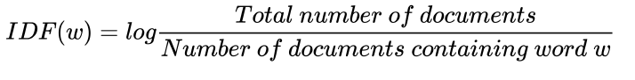
Just like with TD there are many ways to compute IDF, and the most commonly used one is given above. The formula shows that calculating the log gives us the inverse frequency we need.
Combining both the Term Frequency and Inverse Document Frequency we get a final formula that forms the basis of the working of the TF-IDF model.
The TF-IDF formula is given as
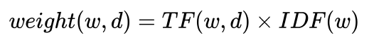
As shown in the above formula, the weight of the word w in document d is given by first calculating the Term Frequency of that word in the document and then calculating the Inverse Document Frequency of the word in the corpus.
Now that we know the working and benefits of using the TF-IDF approach, let’s see how can use the scikit-learn library to create TF-IDF vectors of our text data.
TF-IDF using scikit-learn
Just like CountVectorizer, the scikit-learn library provides a tool to perform TD-IDF vectorization. That tool is the TfidfVectorizer.
We begin by importing the necessary libraries and packages. Run the following lines of code do all the necessary imports.
import numpy as np
import pandas as pd
from sklearn.feature_extraction.text import TfidfVectorizer
We will use the same sample text we had used for CounVectorizer. We define the text and assign it to a variable.
text = (''' Tesla, Inc. is an American electric vehicle and clean energy company based in Palo Alto, California.
        Tesla's current products include electric cars, battery energy storage from
        home to grid-scale, solar panels and solar roof tiles, as well as other related products and services.
        ''')
Next, we convert the text to a Pandas Series object which makes it easier to work with text data. We do this in the code below.
corpus = pd.Series(text)Now we initialize the TfidfVectorizer we had previously imported. After initializing we pass our text data to the vectorizer and the vectorizer transforms the data to a TF-IDF vector. This is done by using the fit_transform method.
vectorizer = TfidfVectorizer()
tf_idf_matrix  = vectorizer.fit_transform(corpus)
Now our vectorized matrix is ready. We print this matrix to check its type.
tf_idf_matrix

Output:
<1x36 sparse matrix of type class numpy.float64 with 36 stored elements in Compressed Sparse Row format>
We see that it is a sparse matrix. If you observe the output message, it shows that the sparse matrix is a type of NumPy array with values of float64 type. So our vectors by definition are a one-dimensional array.
Now we quickly check out the feature names i.e. the words in our vocabulary. To do so run the following line of code.
feature_names

Output:
['alto',
 'american',
 'an',
 'and',
 'as',
 'based',
 'battery',
 'california',
 'cars',
...
From the output, we see the words contained in our vocabulary. Notice that no words are repeated.
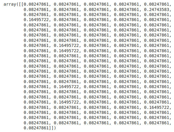
Now if we want to observe the mathematical representation of our text i.e. the TF-IDF representation we have to convert the sparse matrix to a dense matrix. This is done by using the toarray() method. This is done in the code snippet below.
feature_array = tf_idf_matrix.toarray()
feature_array

Output:
array([[0.12700013, 0.12700013, 0.12700013, 0.38100038, 0.25400025, 0.12700013, 0.12700013, 0.12700013,
              0.12700013, 0.12700013, 0.12700013, 0.12700013, 0.25400025, 0.25400025, 0.12700013, 0.12700013,
              0.12700013, 0.12700013, 0.12700013, 0.12700013, 0.12700013, 0.12700013, 0.12700013, 0.12700013,
              0.25400025, 0.12700013, 0.12700013, 0.12700013, 0.12700013, 0.25400025, 0.12700013, 0.25400025,
              0.12700013, 0.12700013, 0.12700013, 0.12700013]])
Observe the output array. This is the mathematical representation of our text.
One difference between the CountVectorizer output and the TF-IDF output to note is that the CountVectorizer outputs were integers, there was no decimal point there. Here in the TD-IDF representation, we see float values. The numbers have a decimal point followed by other numbers.
This signifies that the BoW model just counts the occurrences of words in the text and counts can only be whole numbers, it cannot contain fractions. Whereas here in TF-IDF we are calculating the ratios and logarithms hence we get fractions although we may get a whole number once in a while.
We now print the shape of our matrix. We do so by running the following code.
print(tf_idf_matrix.toarray().shape)

Output:
(1, 36)
Till now we have been tokenizing single words or a single gram. If you check the above feature names, all the terms are single tokens. Take the term “book-keeper”, which is made up of two tokens but conveys a separate meaning altogether when combined. This is called a bigram.
N-gram means n number of continuous tokens taken together as a term. Here, n is the number of tokens. For example, “book” is a one-gram, “book-keeper” is a bi-gram, and so on. N-grams helps us to capture the meaning of such terms in the text. Without N-grams “book” and “keeper” would be taken separately, thus not giving us the desired output.
We now modify the code a little to include a range of grams ranging from one to three. So, we will be including all the terms from one-gram to tri-grams. While initializing the vectorizer, we can define the range of N-grams we want to include.
vectorizer_ngram_range = TfidfVectorizer(analyzer='word', ngram_range=(1,3))Now, we fit this vectorizer to our text data in the first line. In the second line, we get the feature names and print them out in the last line.
bow_matrix_ngram = vectorizer_ngram_range.fit_transform(corpus)
n_gram_feature_names = (vectorizer_ngram_range.get_feature_names()).
n_gram_feature_names
The output is as follows.
['alto',
 'alto california',
 'alto california tesla',
 'american',
 'american electric',
 'american electric vehicle',
 'an',
 'an american',
 'an american electric',
 'and',
The output is exactly as we wanted it to be. It consists not only of one-grams but also of bi-grams and tri-grams. This will help our model to better understand the data. This is our vocabulary and since it consists of tokens till tri-grams, the size of our vocabulary will increase.
Now to see the TF-IDF representation of the above vocabulary, we need to convert the sparse matrix to a dense one and print it out. We do this using the following line of code.
n_gram_feature_array = bow_matrix_ngram.toarray()
n_gram_feature_array
The output is as follows.
The output shows the mathematical representation of the N-gram vocabulary.
We quickly check the size of the vocabulary.
n_gram_feature_array.shape

Output:
(1, 121)
There are 121 total elements in this representation.
Final Thoughts
In this article, we saw some drawbacks of the BoW model and how TF-IDF tries to overcome them. We also went through the working of the model and did it practically using the scikit-learn library. Thanks for reading.